Linear- and Multiple Regression from scratch


You can find working code examples (including this one) in my lab repository on GitHub.
Linear Regression is one of the basic Machine Learning algorithms every student eventually encounters when starting to dive deeper into the field. If you heard someone trying to "fit a line through the data" that person most likely worked with a Linear Regression model.
In which scenarios should we use Linear Regression and if we do, how do we find such a best-fitting line? And what if our data is multidimensional? Let's answer all those questions by implementing Linear and Multiple Regression from scratch!
Note: Throughout this post we'll be using the "Auto Insurance in Sweden" data set which was compiled by the "Swedish Committee on Analysis of Risk Premium in Motor Insurance".
Data-driven decision making
Let's take a step back for a minute and imagine that we're working at an insurance company which sells among other things car insurances.
Over the years the insurance company has collected a wide variety of statistics for all the insurances it sells including data for its car insurances. Some of this data is statistics about the number of filed claims and the payments which were issued for them. The following table shows an excerpt from such data:
| Number of claims | Payments issued |
|---|---|
| 108 | 392,5 |
| 19 | 46,2 |
| 13 | 15,7 |
| 124 | 422,2 |
| ... | ... |
One day we get a call from our colleague who works at the claims settlement center. She has to plan the divisions budget for the upcoming year which is usually derived based on best guesses. Since we've collected all the data throughout the years she wonders if there's a more reliable, mathematical way we could use to calculate the budget estimation.
Nodding along we confirm that we'll dive deeper into this topic and hang up the telephone in sheer excitement! Finally we're able to put some real Machine Learning into practice. But how should we tackle the problem?
Data visualization
It's hard to gain any insights into the data we're dealing with by manually examining the raw numbers. In order to get a better understanding of the data it's always a good idea to visualize it first.
Given that we're dealing with 2 dimensions (the number of claims and the issued payments) one of the potential diagrams we can create is a so called scatter plot which uses (Cartesian) coordinates to display the values of a given data set. In our case we treat the number of claims as our -axis and the issued payments as our -axis and plot the data we recorded at the intersections of such axes which results in the following diagram:
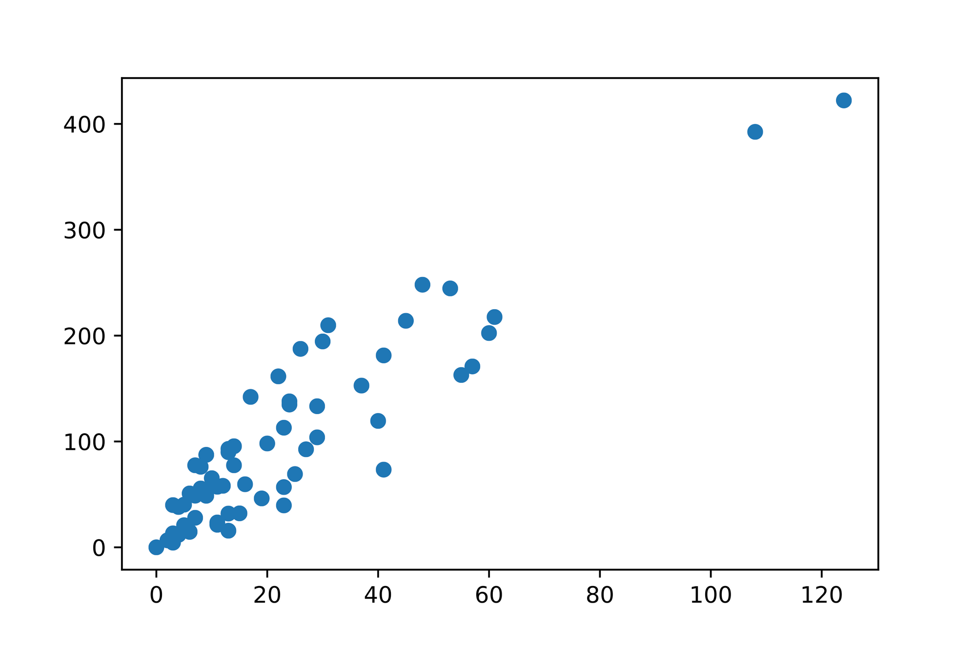
Solely by looking at the diagram we can already identify a trend in the data. It seems to be the case that the more claims were filed, the more payments were issued. Intuitively that makes sense.
After inspecting the plotted data in more detail we observe that we can certainly make some rough predictions for missing data points. Given the trend in the data it seems reasonable that we might issue ~80 payments when ~40 number of claims were filed. Accordingly ~125 claims might be filed when we issue ~410 payments.
Is there some way to turn this insight into a model we can use to make arbitrary predictions? It seems like the relationship in the data is linear. Is there a way to capture this notion mathematically?
Linear Functions
You might remember the concept of a Linear function from school where you've used the slope-intercept form (one of many forms) to mathematically describe a line:
The slope-intercept form has 2 parameters which determine how the line "behaves" in the Cartesian plane (The typical 2D plane with and coordinates):
- is the lines slope which measures how steep the line is slanted
- is the -intercept and determines at which point the line intercepts the -axis
Using this formula we can plug in any arbitrary value which is then multiplied by and added to to get back the corresponding value.
Let's look at a couple of examples to get a better feeling as to how the slope-intercept form works.
The slope m
Let's solely focus on for now and set to . How does influence the way our line will be plotted if we set it to ?
Here's the mathematical representation of such a line followed by the corresponding plot:
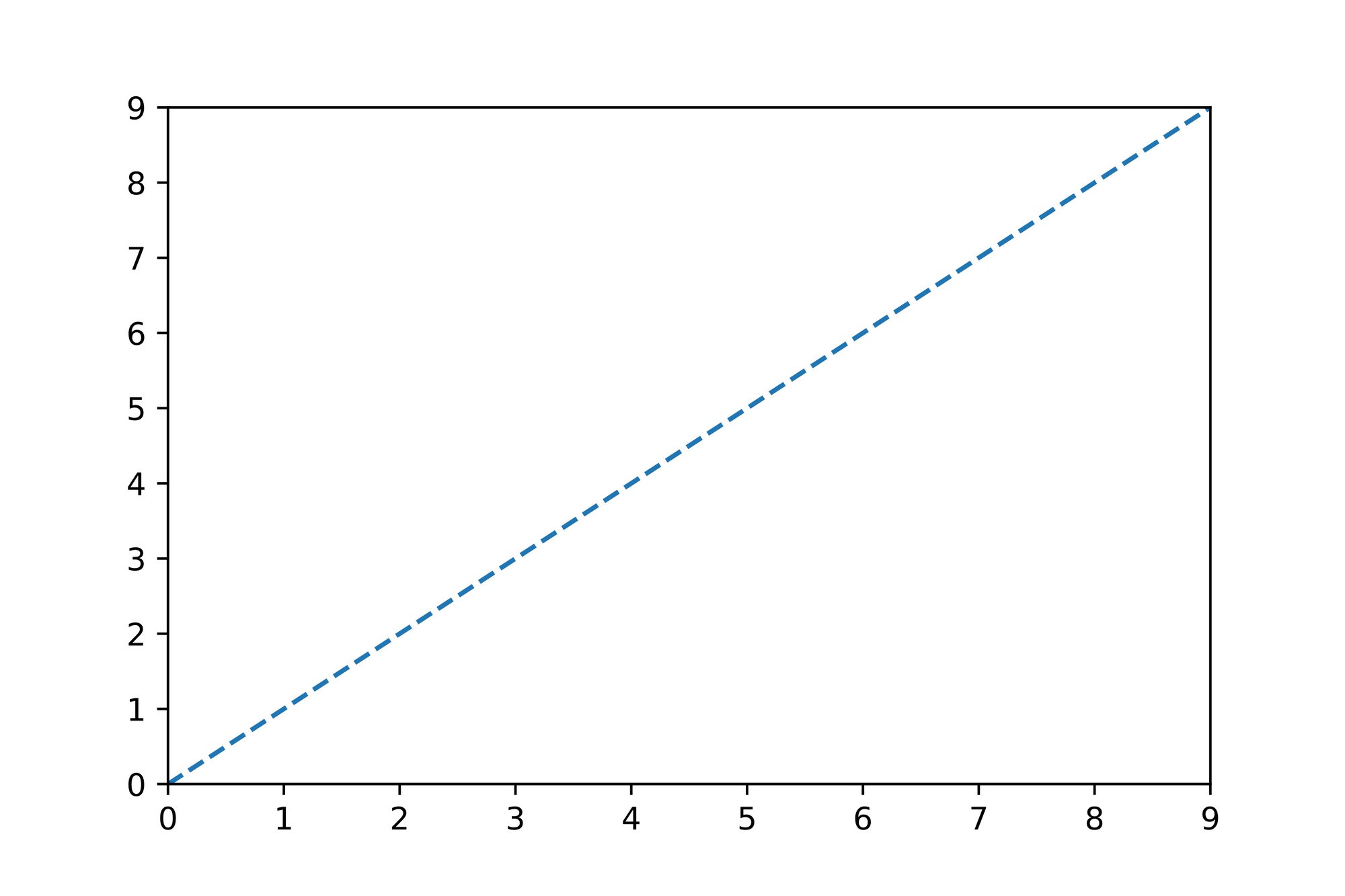
As you can see for every step of size in the direction we "go" a step of size in the direction.
The y-intercept b
Now that we understand what the parameter is responsible for, let's take a look at the -intercept and set it to :
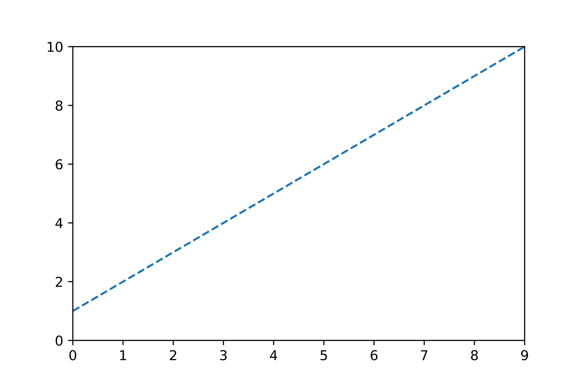
The steepness of the line is the same as the previous line since we haven't modified . However if you take a look at you'll notice that the line crosses the intercept at . That's exactly what the parameter is responsible for. Through we can control where our line should start on the axis when .
Turning it into code
Let's translate the slope-intercept form into a function we call predict (we'll use this function for our predictions later on):
def predict(m: float, b: float, x: float) -> float:
    return m * x + b

assert predict(m=0, b=0, x=3) == 0
Applying what we've learned so far
Let's put the theory into practice and try to guesstimate a line which best describes our data.
The first thing we notice is that the individual data points follow an upwards trend, so will certainly be positive. Furthermore the data points close to seem to have low values as well. Taking those observations into account we guess the following description for our line:
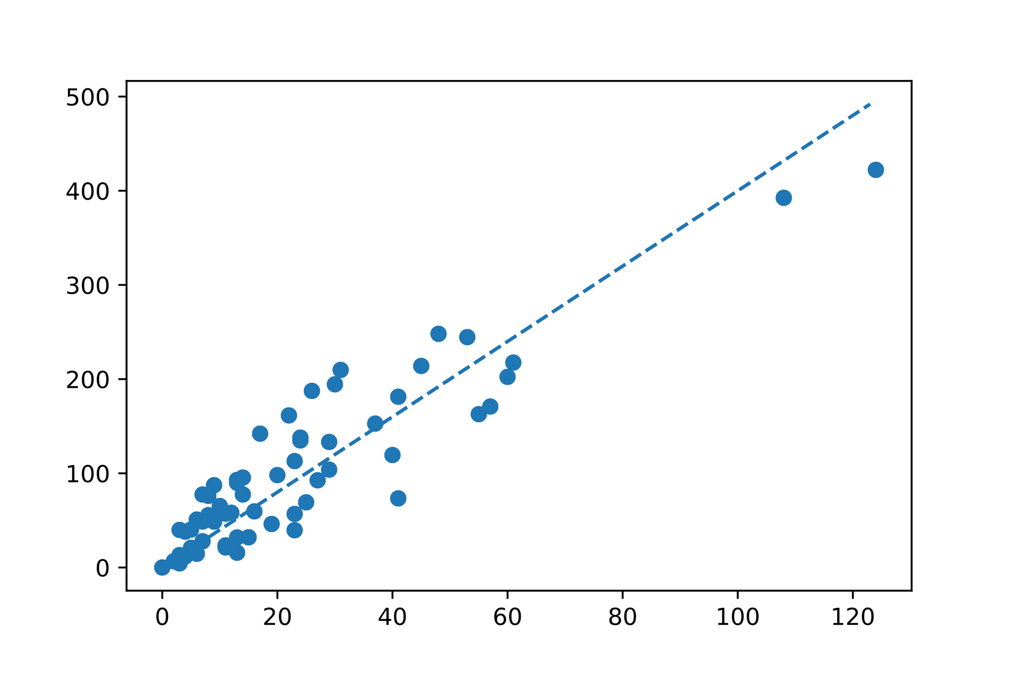
Not too bad for our first guess! Just by looking at the plotted line we might ask ourselves if there's better fitting line? Can we quantify how good our line fits the data?
The error function
Given that the learning part in Machine Learning is usually an iterative process which starts with an initial guess and slowly computes new "best guesses" to finally converge to the optimal solution it's a necessity to be able to track the learning process.
A good way to supervise the learning process is to mathematically capture the "wrongdoing" our algorithm inevitably produces while trying to determine the function which best describes the data.
In the case of Linear Regression it seems to make sense to compare the -values the line produces to the actual -values from the data set. We could for example go through each individual pair in our data set and subtract its value from the value our line "predicts" for the corresponding . Summing up these differences results in a number we can use to compare different lines against each other. The higher the number, the "less correct" the line.
That's great but there's one minor catch. Imagine that the line which is fitted through the data predicts large positive values near the origin where it should predict large negative numbers. At the same time it predicts large negative numbers near the end of the -axis although those values should be positive. If we calculate the errors according to our description above where we suggested to sum up the differences between the values we'd end up in a situation where values might cancel each other out. In the worst case the calculated error is which indicates that we've found the best fitting line while in reality we didn't!
A simple trick to mitigate this problem is to square each single error value before they're summed up. This way any negative value will be turned into a positive one, making it impossible to run into scenarios where error calculations cancel each other out.
The error function we've just described is called Residual sum of squares (RSS) or Sum of squared errors (SSE) and is one of many error functions we can use to quantify the algorithms "wrongdoing". The following is the mathematical formula for SSE:
Turing that into code results in the following:
def sum_squared_error(ys: List[float], ys_pred: List[float]) -> float:
    assert len(ys) == len(ys_pred)
    return sum([(y - ys_pred) ** 2 for y, ys_pred in zip(ys, ys_pred)])

assert sum_squared_error([1, 2, 3], [4, 5, 6]) == 27
Finding the best fitting line...
With those two code snippets (the predict and sum_squared_error functions) we're now able to describe a line, predict values and measure how "off" our predictions are. The last missing piece we'll need to get in place is a way to update our line description such that the next sum_squared_error calculation returns an error value which is less than our current one. If there's a way to constantly reduce the error we're making by slowly updating our line description we'll eventually end up with a line which best fits our data!
With Linear Regression there are a couple of different algorithms we can use to find the best fitting line. One prominent choice is the Ordinary least squares (OLS) method. Since OLS is a common choice we'll do something different. We'll use the Gradient Descent algorithm which can be used for various different optimization problems and is at the heart of modern Machine Learning algorithms.
Note: If you haven't already I'd suggest that you take a couple of minutes to read the article "Gradient Descent from scratch" in which I explain the whole algorithm in great detail.
... using Gradient Descent
I won't provide too many explanations regarding Gradient Descent here since I already covered the topic in the aforementioned post. Don't get too intimidated by the Math below. It's ok if you just skim through this section to get a high-level overview.
In a nutshell Gradient Descent makes it possible for us to iteratively "walk down" the error functions surface to eventually find a local minimum where the error is the smallest which is exactly what we're looking for.
In order to figure out in which direction we should walk to descent down to the local minimum we need to compute the so-called gradient. The gradient is a vector consisting of partial derivatives of our error function which point in the direction of greatest increase at any given point on our error functions surface.
To find the partial derivatives of our SSE function we should expand it so that we can see all the variables we need to take into account:
Looking at the expanded formula it seems like there's and we need to derive with respect to:
Which results in the following code:
# The partial derivative of SSE with respect to `m`
grad_m: float = sum([2 * (predict(m, b, x) - y) * x for x, y in zip(xs, ys)])
# The partial derivative of SSE with respect to `b`
grad_b: float = sum([2 * (predict(m, b, x) - y) for x, y in zip(xs, ys)])
Tip: You can use WolframAlpha to validate your partialderivatives.
Given these partial derivatives we can now calculate the gradient for any point which is a vector pointing in the direction of greatest increase. Multiplying the vector by will let it point into the opposite direction, the direction of greatest decrease (remember that we want to find a local minimum). If we add a small fraction of this vector to our and values respectively we should end up closer to a local minimum.
The following code captures what we've just described:
# Take a small step in the direction of greatest decrease
# The `learning_rate` controls the step size when "walking" down the gradient
learning_rate: float = 0.0001

m = m + (grad_m * -1 * learning_rate)
b = b + (grad_b * -1 * learning_rate)
Repeating this process multiple times should help us find the and values for our line for which any given prediction calculated by that line results in the smallest error possible.
Let's put all the pieces together and implement the Gradient Descent algorithm to find the best fitting line:
# Find the best fitting line through the data points via Gradient Descent

# Our initial guess
m: float = 0
b: float = 200

print(f'Starting with "m": {m}')
print(f'Starting with "b": {b}')

# Doing 1000 iterations
epochs: int = 10000
learning_rate: float = 0.00001

for epoch in range(epochs):
    # Calculate predictions for `y` values given the current `m` and `b`
    ys_pred: List[float] = [predict(m, b, x) for x in xs]

    # Calculate and print the error
    if epoch % 1000 == True:
        loss: float = sum_squared_error(ys, ys_pred)
        print(f'Epoch {epoch} --> loss: {loss}')

    # Calculate the gradient
    # Taking the (partial) derivative of SSE with respect to `m` results in `2 * x ((m * x + b) - y)`
    grad_m: float = sum([2 * (predict(m, b, x) - y) * x for x, y in zip(xs, ys)])
    # Taking the (partial) derivative of SSE with respect to `b` results in `2 ((m * x + b) - y)`
    grad_b: float = sum([2 * (predict(m, b, x) - y) for x, y in zip(xs, ys)])

    # Take a small step in the direction of greatest decrease
    m = m + (grad_m * -learning_rate)
    b = b + (grad_b * -learning_rate)

print(f'Best estimate for "m": {m}')
print(f'Best estimate for "b": {b}')
Running this algorithm results in a best estimate for the and values. Let's compare our initial guess of and (the guess we started with at the top of the code snippet) with the values our Gradient Descent implementation produced:
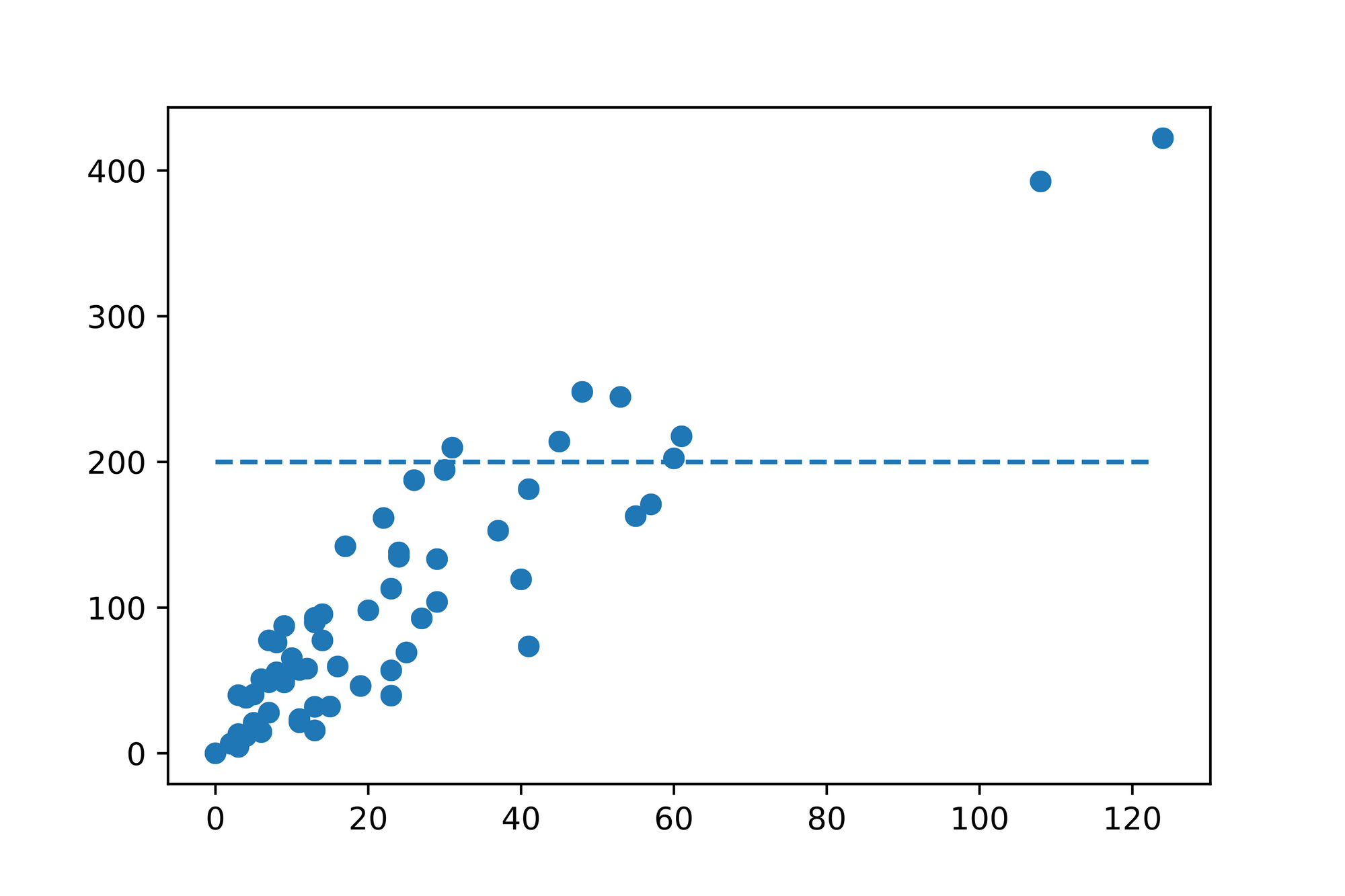
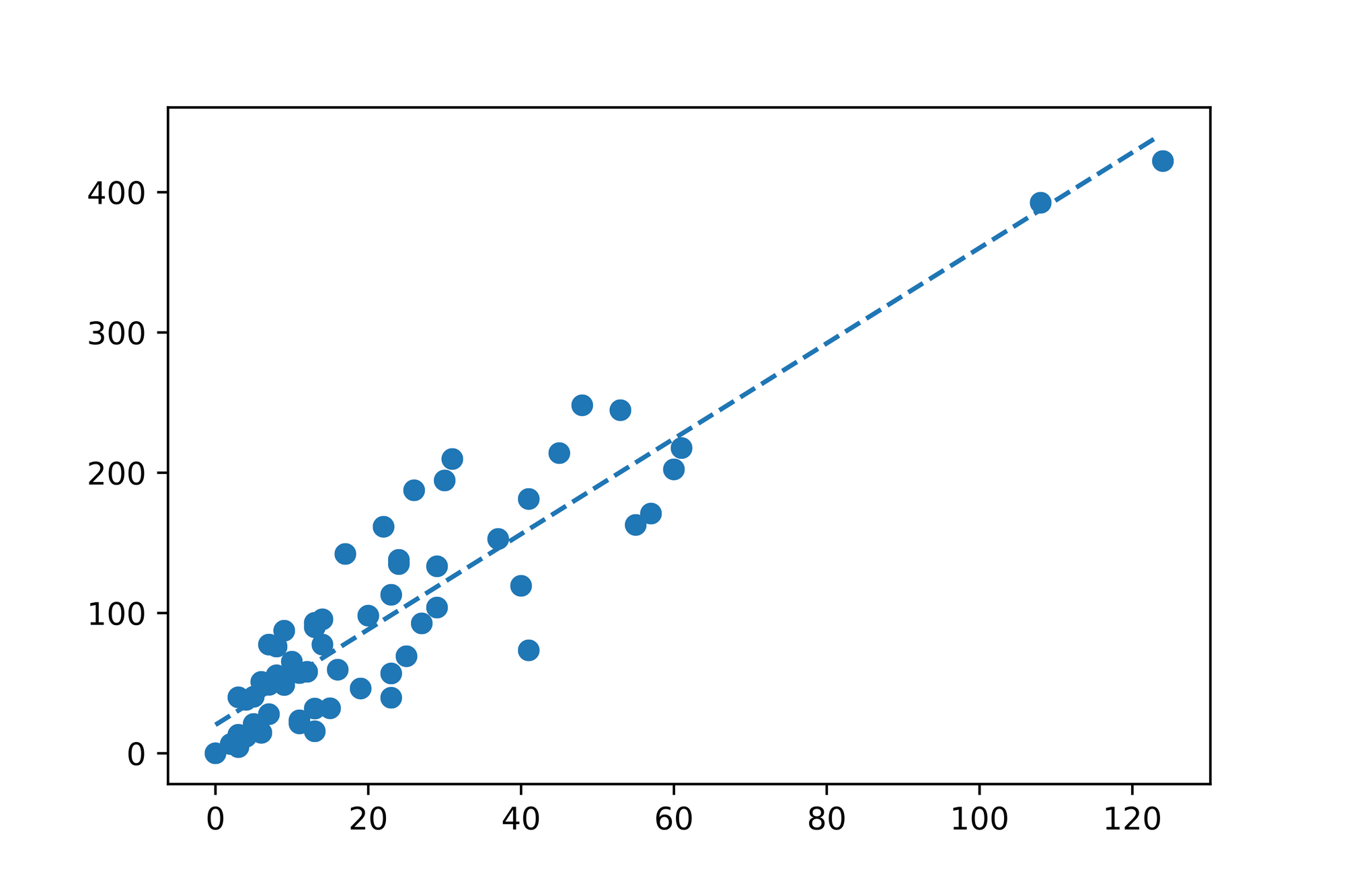
Awesome! Seems like we've found our linear function which best describes our data! Let's call our co-worker and share the good news. From now on she can use the following formula to find a prediction for the issued payments () based on any number of claims ():
From Linear Regression to Multiple Regression
It's great to be able to fit a line through data points in dimensions. But how do we deal with scenarios where our data has more than dimensions?
Most data sets capture many different measurements which are called "features". It would be great if we could take the most important features into account when working with our algorithms. Given that every feature adds another dimension we need to ensure that the model we're building can deal with such high-dimensional data.
Our Linear Regression model was only able to take a single value and predict a corresponding value. What if we have multiple values? Is there a way to use a regression model to predict a value based on multiple values?
As it turns out Linear Regression is a subset of a general regression model called Multiple Linear Regression or Multiple Regression. Multiple Regression can deal with an arbitrary number of values expressed as a vector to predict a single value.
The great news is that we can easily adopt what we've learned so far to deal with high-dimensional data. Let's take a quick look at the changes we need to make.
Tweaking the Linear Function
The slope-intercept form we've used so far can easily be updated to work with multiple values. Here's the linear equation we've used so far:
Having multiple values means that we'll also have multiple values (one for each ). However we'll still only deal with intercept:
Calculating a prediction for is as simple as solving the above equation for any given vector of values, vector of values and any given value.
There's one little trick we can apply given that we're now mostly dealing with vectors rather than scalar numbers. To make the computation more efficient we can use the dot-product which carries out almost the exact same calculation we described above. There's just one problem. The dot-product can only be used in vector calculations, however isn't a vector. As it turns out we can simply prepend the value to the vector and prepend a to the vector. Doing this little trick makes it possible to use the dot-product calculation while also taking the value into account. Here's what we'd end up with when doing just that:
Another nice side-effect of doing this is that the partial derivative calculations for the error function will also be easier since our usage of the dot-product reduced the number of variables we have to take into account to just 2 vectors and .
Fitting Hyperplanes
And that's pretty much all there is to change. The rest of the code follows exactly the same way. While we fitted a line when working with Linear Regression we're now fitting a so-called hyperplane with Multiple Regression.
To get a better intuition for the notion of a hyperplane imagine that we have measurements we can scatter plot in a dimensional space. Every measurement will be a single dot in that space, resulting in a cloud of dots. Our Multiple Regression algorithm will now try to find a plane (think of it as a wooden plank) which best fits through that dot cloud.
Conclusion
Linear Regression is one of the very first algorithms every student encounters when learning about Machine Learning models and algorithms.
The basic idea of Linear Regression is to find an equation for a line which best describes the data points in the given data set. Such a line is often described via the point-slope form . "Fitting the line" means finding the and values such that the resulting value is as accurate as possible given an arbitrary value. Using an error function (which describes how "off" our current line equation is) in combination with an optimization algorithm such as Gradient Descent makes it possible to iteratively find the "best fitting" line.
As it turns out Linear Regression is a specialized form of Multiple Linear Regression which makes it possible to deal with multidimensional data by expressing the and values as vectors. While this requires the usage of techniques such as the dot-product from the realm of Linear Algebra the basic principles still apply. In Multiple Linear Regression we're just trying to find a "best fitting" hyperplane rather than a line.
Do you have any questions, feedback or comments? Feel free to reach out via E-Mail or connect with me on Twitter.
Additional Resources
The following is a list with resources I've used while working on this blog post. Other useful resources are linked within the article itself.