K-nearest neighbors from scratch

You can find working code examples (including this one) in my lab repository on GitHub.

K-nearest neighbors (abbreviated as k-NN or KNN) is a simple, yet elegant Machine Learning algorithm to classify unseen data based on existing data. The neat property of this algorithm is that it doesn't require a "traditional" training phase. If you have a classification problem and labeled data you can predict the class of any unseen data point by leveraging your existing, already classified data.

Let's take a closer look at the intuitions behind the core ideas, the involved math and the translation of such into code.

The intuition

Imagine that we've invited 100 dog owners with their dogs over for a statistical experiment we want to run. Each dog participating in this experiment is 1 out of 4 different dog breeds we're interested in studying. While we have the dog owners and their dogs around we measure 3 different properties of each dog:

• Its weight (in kilograms)
• Its height (in centimeters)
• Its alertness (on a scale from 0 to 1 [1=very alert, 0=almost no alertness])

Once done, we normalize the measurements so that they fall into a range between $0$ and $1$.

After collection the data on each individual dog we end up with 100 3-pair measurements, each of which is labeled with the corresponding dog breed.

Here's one example:

In order to better understand the data it's always a good idea to plot it. Since we have collected 3 different measurements (weight, height and alertness) it's possible to project all of the 100 data points into a 3 dimensional space and color every data point according to its label (e.g. brown for the label "Podenco").

Unfortunately we run into an issue while attempting to plot this data. As it turns out we forgot to label one measurement. We do have the dogs width, its height and its alertness but for some reason we forgot to write down the dogs breed.

Is there any chance we could derive what this dogs breed might be given all the other dog measurements we already have? We can still add the unlabeled data point into our existing 3 dimensional space where all the other colored data points reside. But how should we color it?

One potential solution is to look at the, say 5 surrounding neighbors of the data point in question and see what their color is. If the majority of those data points is labeled "Podenco" then it's very likely that our measurements were also taken from a Podenco.

And that's exactly what the k-NN algorithm does. The k-nearest neighbors algorithm predicts the class of an unseen data point based on its k-nearest neighbors and the majority of their respective classes. Let's take a closer look at this from a mathematical perspective.

The 2 building blocks

There are only 2 concepts we need to implement in order to classify unseen data via k-NN.

As stated above, the algorithm works by looking at the k-nearest neighbors and the majority of their respective classes in order to classify unseen data.

Because of that we need to implement 2 functions. A distance function which calculates the distance between two points and a voting function which returns the most seen label given a list of arbitrary labels.

Distance function

Given the notion of "nearest neighbors" we need to calculate the distance between our "to be classified" data point and all the other data points to find the $k$ closest ones.

There are a couple of different distance functions out there. For our implementation we'll use the Euclidean distance as it's simple to calculate and can easily scale up to $n$ dimensions.

The mathematical notation is as follows:

Let's unpack this formula with the help of an example. Assuming we have two vectors $a$ and $b$, the euclidean distance between the two is calculated as follows:

Translating this into code results in the following:

def distance(x: List[float], y: List[float]) -> float:
    assert len(x) == len(y)
    return sqrt(sum((x[i] - y[i]) ** 2 for i in range(len(x))))

assert distance([1, 2, 3, 4], [5, 6, 7, 8]) == 8

Great. We just implemented the first building block: An Euclidean distance function.

Voting function

Next up we need to implement a voting function. The voting function takes as an input a list of labels and returns the "most seen" label of that list. While this sounds trivial to implement we should take a step back and think about potential edge cases we might run into.

One of those edge cases is the situation in which we have 2 or more "most seen" labels:

# Do we return `a` or `b`?
labels: List[str] = ['a', 'a', 'b', 'b', 'c']

For those scenarios we need to implement a tie breaking mechanism.

There are several ways to deal with this. One solution might be to pick a candidate randomly. In our case however we shouldn't think about the vote function in isolation since we know that the distance and vote functions both work together to determine the label of the unseen data point.

We can exploit this fact and assume that the list of labels our vote function gets as an input is sorted by distance, nearest to furthest. Given this requirement it's easy to break ties. All we need to do is recursively remove the last entry in the list (which is the furthest) until we only have one clear winning label.

The following demonstrates this process based on the labels example from above:

# Do we return `a` or `b`?
labels: List[str] = ['a', 'a', 'b', 'b', 'c']

# Remove one entry. We're still unsure if we should return `a` or `b`
labels: List[str] = ['a', 'a', 'b', 'b']

# Remove another entry. Now it's clear that `a` is the "winner"
labels: List[str] = ['a', 'a', 'b']

Let's translate that algorithm into a function we call majority_vote:

def majority_vote(labels: List[str]) -> str:
    counted: Counter = Counter(labels)
    winner: List[str] = []
    max_num: int = 0
    most_common: List[Tuple[str, int]]
    for most_common in counted.most_common():
        label: str = most_common[0]
        num: int = most_common[1]
        if num < max_num:
            break
        max_num = num
        winner.append(label)
    if len(winner) > 1:
        return majority_vote(labels[:-1])
    return winner[0]

assert majority_vote(['a', 'b', 'b', 'c']) == 'b'
assert majority_vote(['a', 'b', 'b', 'a']) == 'b'
assert majority_vote(['a', 'a', 'b', 'b', 'c']) == 'a'

The tests at the bottom show that our majority_vote function reliably deals with edge cases such as the one described above.

The k-NN algorithm

Now that we've studied and codified both building blocks it's time to bring them together. The knn function we're about to implement takes as inputs the list of labeled data points, a new measurement (the data point we want to classify) and a parameter k which determines how many neighbors we want to take into account when voting for the new label via our majority_vote function.

The first thing our knn algorithm should do is to calculate the distances between the new data point and all the other, existing data points. Once done we need to order the distances from nearest to furthest and extract the data point labels. This sorted list is then truncated so that it only contains the k nearest data point labels. The last step is to pass this list into the voting function which computes the predicted label.

Turning the described steps into code results in the following knn function:

def knn(labeled_data: List[LabeledData], new_measurement, k: int = 5) -> Prediction:
    class Distance(NamedTuple):
        label: str
        distance: float
    distances: List[Distance] = [Distance(data.label, distance(new_measurement, data.measurements))
                                          for data in labeled_data]
    distances = sorted(distances, key=attrgetter('distance'))
    labels = [distance.label for distance in distances][:k]
    label: str = majority_vote(labels)
    return Prediction(label, new_measurement)

That's it. That's the k-nearest neighbors algorithm implemented from scratch!

Classifying Iris flowers

It's time to see if our homebrew k-NN implementation works as advertised. To test drive what we've coded we'll use the infamous Iris flower data set.

The data set consists of 50 samples of three different flower species called Iris:

• Iris Setosa
• Iris Virginica
• Iris Versicolor

For each sample, 4 different measurements were collected: The sepal width and length as well as its petal width and length.

The following is an example row from the data set where the first 4 numbers are the sepal length, sepal width, petal length, petal width and the last string represents the label for those measurements.

6.9,3.1,5.1,2.3,Iris-virginica

The best way to explore this data is to plot it. Unfortunately it's hard to plot and inspect 4 dimensional data. However we can pick 2 measurements (e.g. petal length and petal width) and scatter plot those in 2 dimensions.

Note: We're using the amazing Plotly library to create our scatter plots.

fig = px.scatter(x=xs, y=ys, color=text, hover_name=text, labels={'x': 'Petal Length', 'y': 'Petal Width'})
fig.show()

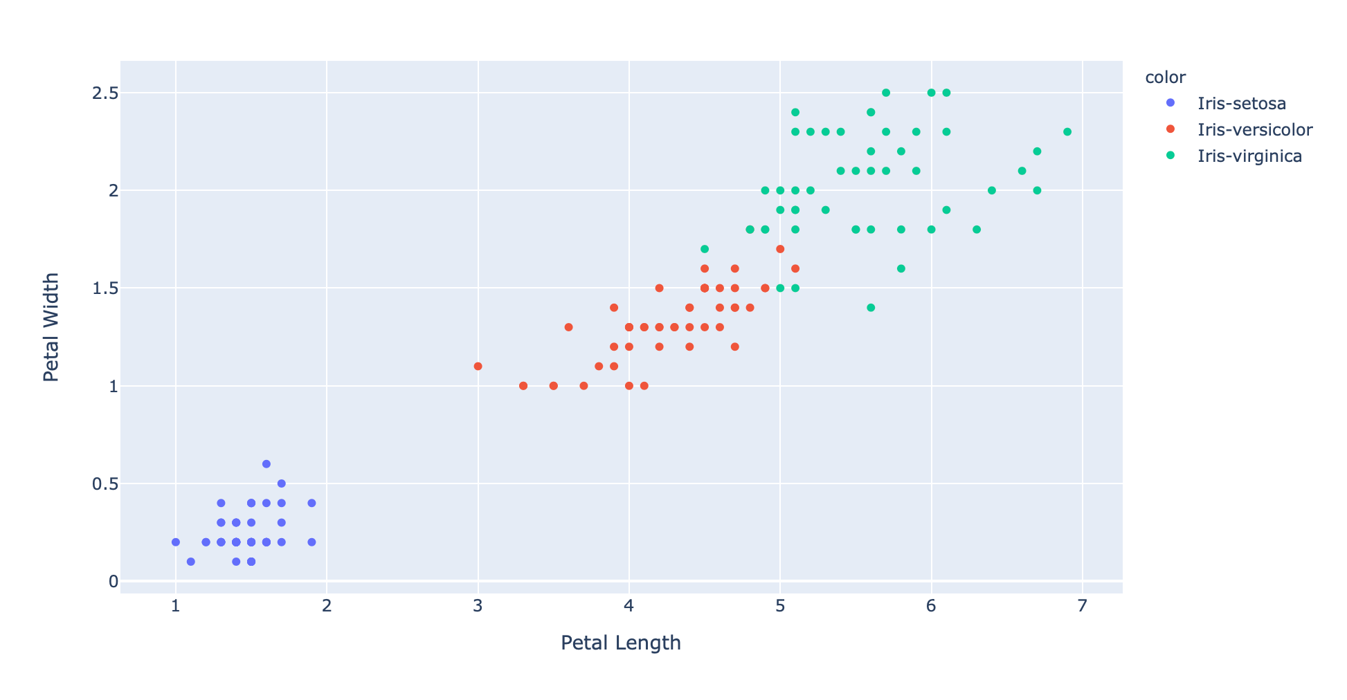We can clearly see clusters of data points which all share the same color and therefore the same label.

Now let's pretend that we have a new, unlabeled data point:

new_measurement: List[float] = [7, 3, 4.8, 1.5]

Adding this data point to our existing scatter plot results in the following:

fig = px.scatter(x=xs, y=ys, color=text, hover_name=text, labels={'x': 'Petal Length', 'y': 'Petal Width'})
fig.add_annotation(
    go.layout.Annotation(
            x=new_measurement[petal_length_idx],
            y=new_measurement[petal_width_idx],
            text="The measurement we want to classify")
)
fig.update_annotations(dict(
            xref="x",
            yref="y",
            showarrow=True,
            arrowhead=7,
            ax=0,
            ay=-40,
            borderwidth=2,
            borderpad=4,
            bgcolor="#c3c3c3"
))
fig.show()

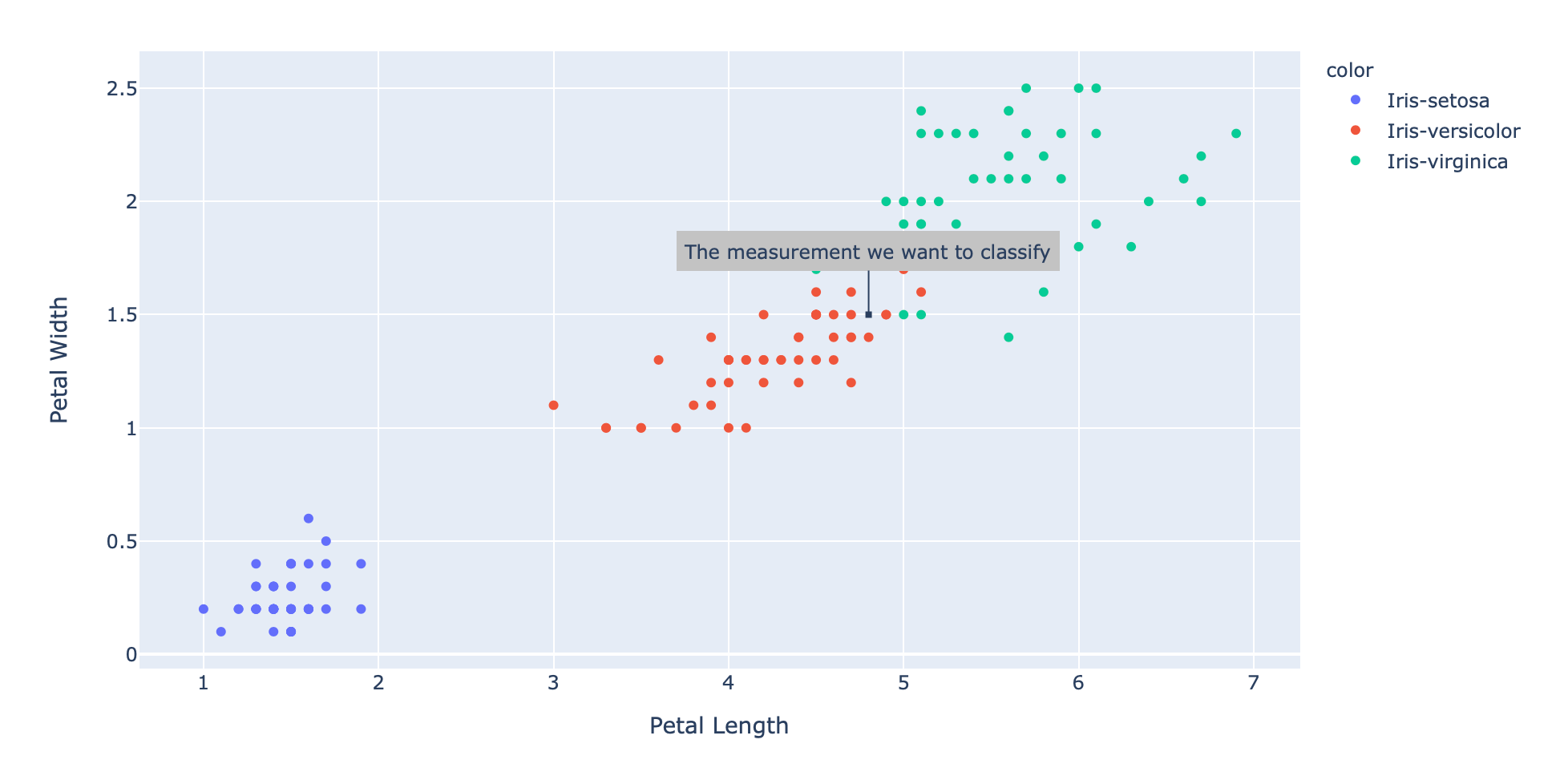Even if we're just plotting the petal length and petal width in 2 dimensions it seems to be the case that the new measurement might be coming from an "Iris Versicolor".

Let's use our knn function to get a definite answer:

knn(labeled_data, new_measurement, 5)

And sure enough the result we get back indicates that we're dealing with an "Iris Versicolor":

Prediction(label='Iris-versicolor', measurements=[7, 3, 4.8, 1.5])

Conclusion

k-nearest neighbors is a very powerful classification algorithm which makes it possible to label unseen data based on existing data. k-NNs main idea is to use the $k$ nearest neighbors of the new, "to-be-classified" data point to "vote" on the label it should have.

Given that, we need 2 core functions to implement k-NN. The first function calculates the distance between 2 data points so that nearest neighbors can be found. The second function performs a majority vote so that a decision can be made as to what label is most present in the given neighborhood.

Using both functions together brings k-NN to life and makes it possible to reliably label unseen data points.

Do you have any questions, feedback or comments? Feel free to reach out via E-Mail or connect with me on Twitter.

Thanks to Eric Nieuwland who reached out via E-Mail and provided some code simplifications!

Additional Resources

The following is a list of resources I've used to work on this blog post. Other helpful resources are also linked within the article itself.

• Joel Grus - Data Science from Scratch
• Wikipedia - k-nearest neighbors algorithm
• Wikipedia - Euclidean distance
• Wikipedia - Iris flower data set
• UCI - Iris Data Set