Minimax and Monte Carlo Tree Search

Do you remember your childhood days when you discovered the infamous game Tic-Tac-Toe and played it with your friends over and over again?

You might've wondered if there's a certain strategy you can exploit that lets you win all the time (or at least force a draw). Is there such an algorithm that will show you how you can defeat your opponent at any given time?

It turns out there is. To be precise there are a couple of algorithms which can be utilized to predict the best possible moves in games such as Tic-Tac-Toe, Connect Four, Chess and Go among others. One such family of algorithms leverages tree search and operates on game state trees.

In this blog post we'll discuss 2 famous tree search algorithms called Minimax and Monte Carlo Tree Search (abbreviated to MCTS). We'll start our journey into tree search algorithms by discovering the intuition behind their inner workings. After that we'll see how Minimax and MCTS can be used in modern game implementations to build sophisticated Game AIs. We'll also shed some light into the computational challenges we'll face and how to handle them via performance optimization techniques.

The Intuition behind tree search

Let's imagine that you're playing some games of Tic-Tac-Toe with your friends. While playing you're wondering what the optimal strategy might be. What's the best move you should pick in any given situation?

Generally speaking there are 2 modes you can operate in when determining the next move you want to play:

Aggressive:

• Play a move which will cause an immediate win (if possible)
• Play a move which sets up a future winning situation

Defensive:

• Play a move which prevents your opponent from winning in the next round (if possible)
• Play a move which prevents your opponent from setting up a future winning situation in the next round

These modes and their respective actions are basically the only strategies you need to follow to win the game of Tic-Tac-Toe.

The "only" thing you need to do is to look at the current game state you're in and play simulations through all the potential next moves which could be played. You do this by pretending that you've played a given move and then continue playing the game until the end, alternating between the X and O player. While doing that you're building up a game tree of all the possible moves you and your opponent would play.

The following illustration shows a simplified version of such a game tree: 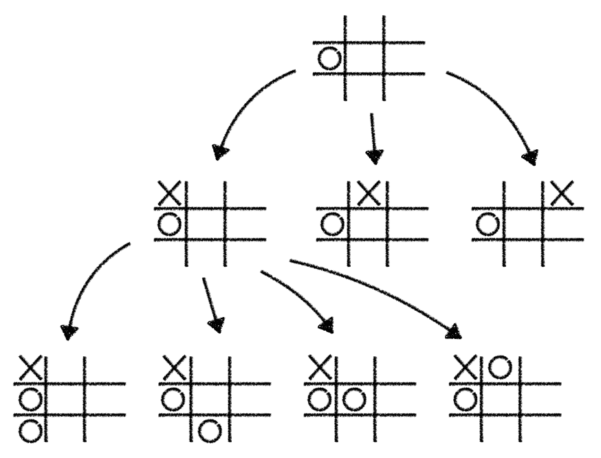Note that for the rest of this post we'll only use simplified game tree examples to save screen space

Of course, the set of strategic rules we've discussed at the top is specifically tailored to the game of Tic-Tac-Toe. However we can generalize this approach to make it work with other board games such as Chess or Go. Let's take a look at Minimax, a tree search algorithm which abstracts our Tic-Tac-Toe strategy so that we can apply it to various other 2 player board games.

The Minimax Algorithm

Given that we've built up an intuition for tree search algorithms let's switch our focus from simple games such as Tic-Tac-Toe to more complex games such as Chess.

Before we dive in let's briefly recap the properties of a Chess game. Chess is a 2 player deterministic game of perfect information. Sound confusing? Let's unpack it:

In Chess, 2 players (Black and White) play against each other. Every move which is performed is ensured to be "fulfilled" with no randomness involved (the game doesn't use any random elements such as a die). During gameplay every player can observe the whole game state. There's no hidden information, hence everyone has perfect information about the whole game at any given time.

Thanks to those properties we can always compute which player is currently ahead and which one is behind. There are several different ways to do this for the game of Chess. One approach to evaluate the current game state is to add up all the remaining white pieces on the board and subtract all the remaining black ones. Doing this will produce a single value where a large value favors white and a small value favors black. This type of function is called an evaluation function.

Based on this evaluation function we can now define the overall goal during the game for each player individually. White tries to maximize this objective while black tries to minimize it.

Let's pretend that we're deep in an ongoing Chess game. We're player white and have already played a couple of clever moves, resulting in a large number computed by our evaluation function. It's our turn right now but we're stuck. Which of the possible moves is the best one we can play?

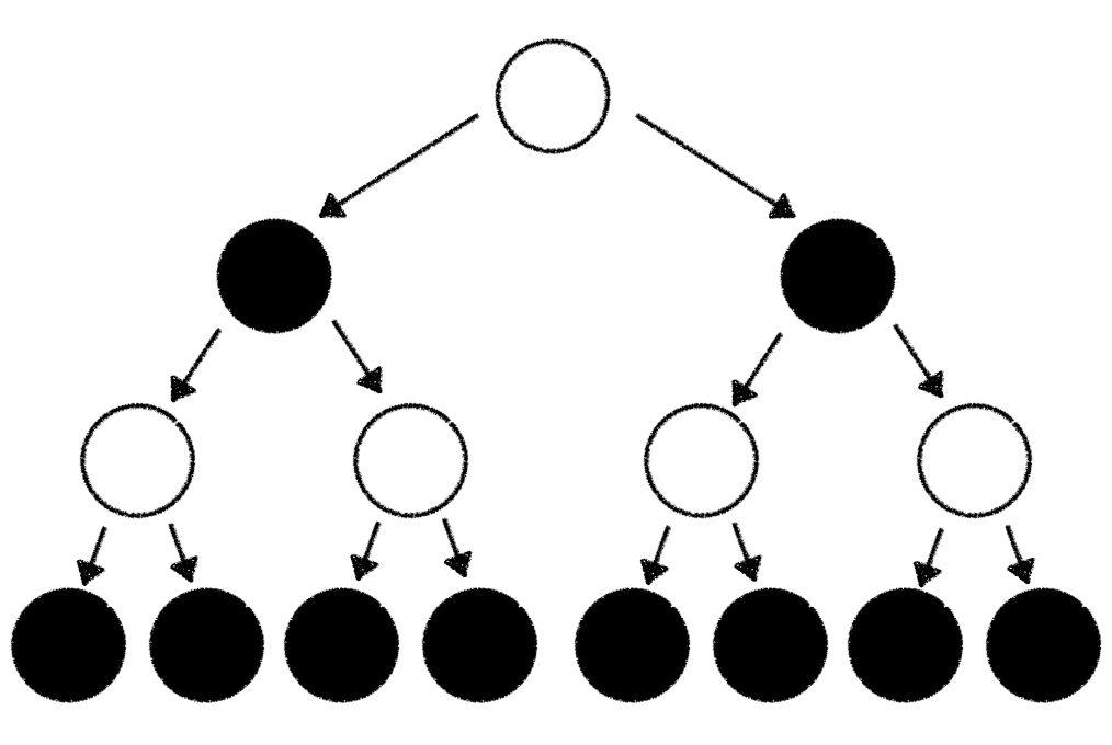
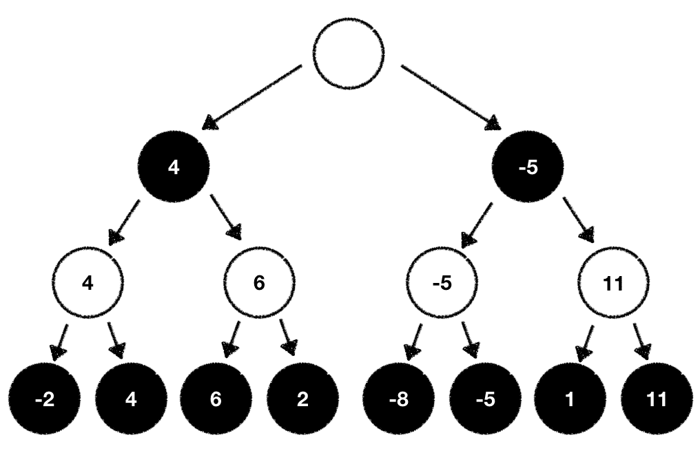
We'll solve this problem with the same approach we already encountered in our Tic-Tac-Toe gameplay example. We build up a tree of potential moves which could be performed based on the game state we're in. To keep things simple we pretend that there are only 2 possible moves we can play (in Chess there are on average ~30 different options for every given game state). We start with a (white) root node which represents the current state. Starting from there we're branching out 2 (black) child nodes which represent the game state we're in after taking one of the 2 possible moves. From these 2 child nodes we're again branching out 2 separate (white) child nodes. Each one of those represents the game state we're in after taking one of the 2 possible moves we could play from the black node. This branching out of nodes goes on and on until we've reached the end of the game or hit a predefined maximum tree depth.

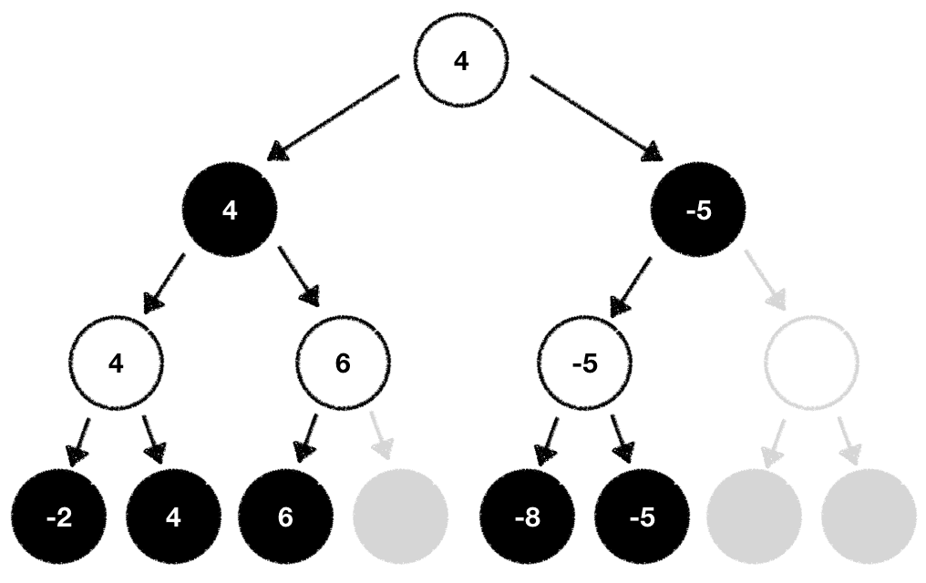
The resulting tree looks something like this:

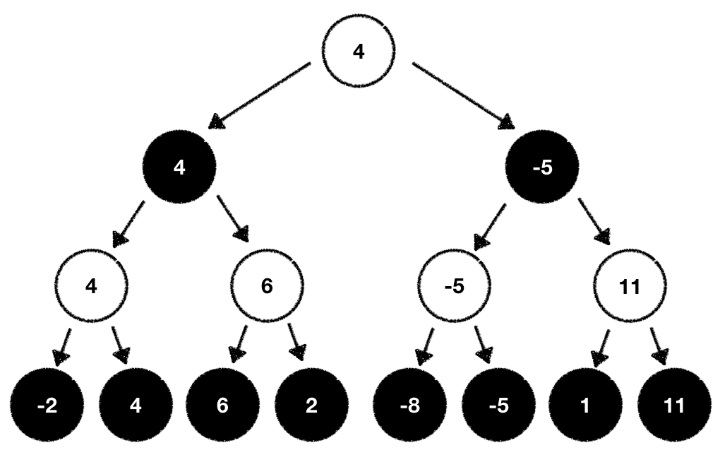
Given that we're at the end of the tree we can now compute the game outcome for each end state with our evaluation function:

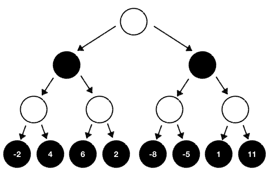
With this information we now know the game outcome we can expect when we take all the outlined moves starting from the root node and ending at the last node where we calculated the game evaluation. Since we're player white it seems like the best move to pick is the one which will set us up to eventually end in the game state with the highest outcome our evaluation function calculated.

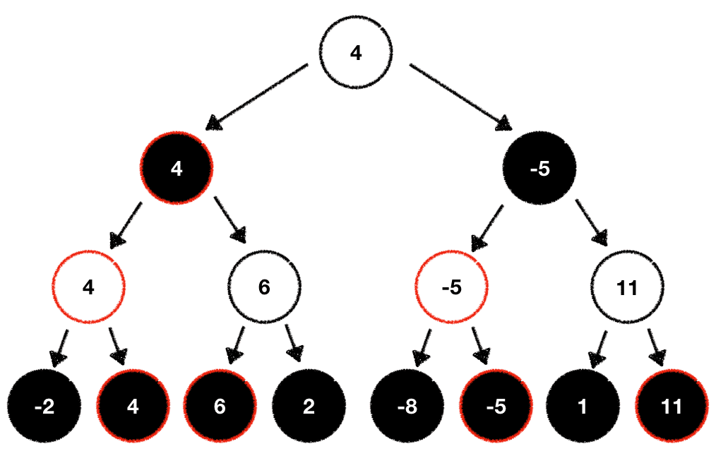
While this is true there's one problem. There's still the black player involved and we cannot directly manipulate what move she'll pick. If we cannot manipulate this why don't we estimate what the black player will likely do based on our evaluation function? As a white player we always try to maximize our outcome. The black player always tries to minimize the outcome. With this knowledge we can now traverse back through our game tree and compute the values for all our individual tree nodes step by step.

White tries to maximize the outcome:

While black wants to minimize it:

Once done we can now pick the next move based on the evaluation values we've just computed. In our case we pick the next possible move which maximizes our outcome:

What we've just learned is the general procedure of the so-called Minimax algorithm. The Minimax algorithm got its name from the fact that one player wants to Mini-mize the outcome while the other tries to Max-imize it.

Code

def minimax(state, max_depth, is_player_minimizer):
    if max_depth == 0 or state.is_end_state():
        # We're at the end. Time to evaluate the state we're in
        return evaluation_function(state)

    # Is the current player the minimizer?
    if is_player_minimizer:
        value = -math.inf
        for move in state.possible_moves():
            evaluation = minimax(move, max_depth - 1, False)
            min = min(value, evaluation)
        return value

    # Or the maximizer?
    value = math.inf
    for move in state.possible_moves():
        evaluation = minimax(move, max_depth - 1, True)
        max = max(value, evaluation)
    return value

Search space reduction with pruning

Minimax is a simple and elegant tree search algorithm. Given enough compute resources it will always find the optimal next move to play.

But there's a problem. While this algorithm works flawlessly with simplistic games such as Tic-Tac-Toe, it's computationally infeasible to implement it for strategically more involved games such as Chess. The reason for this is the so-called tree branching factor. We've already briefly touched on that concept before but let's take a second look at it.

In our example above we've artificially restricted the potential moves one can play to 2 to keep the tree representation simple and easy to reason about. However the reality is that there are usually more than 2 possible next moves. On average there are ~30 moves a Chess player can play in any given game state. This means that every single node in the tree will have approximately 30 different children. This is called the width of the tree. We denote the trees width as $w$.

But there's more. It takes roughly ~85 consecutive turns to finish a game of Chess. Translating this to our tree means that it will have an average depth of 85. We denote the trees depth as $d$.

Given $w$ and $d$ we can define the formula $w^d$ which will show us how many different positions we have to evaluate on average.

Plugging in the numbers for Chess we get $30^{85}$. Taking the Go board game as an example which has a width $w$ of ~250 and an average depth $d$ of ~150 we get $250^{150}$. I encourage you to type those numbers into your calculator and hit enter. Needless to say that current generation computers and even large scale distributed systems will take "forever" to crunch through all those computations.

Does this mean that Minimax can only be used for games such as Tic-Tac-Toe? Absolutely not. We can apply some clever tricks to optimize the structure of our search tree.

Generally speaking we can reduce the search trees width and depth by pruning individual nodes and branches from it. Let's see how this works in practice.

Alpha-Beta Pruning

Recall that Minimax is built around the premise that one player tries to maximize the outcome of the game based on the evaluation function while the other one tries to minimize it.

This gameplay behavior is directly translated into our search tree. During traversal from the bottom to the root node we always picked the respective "best" move for any given player. In our case the white player always picked the maximum value while the black player picked the minimum value: Looking at our tree above we can exploit this behavior to optimize it. Here's how:

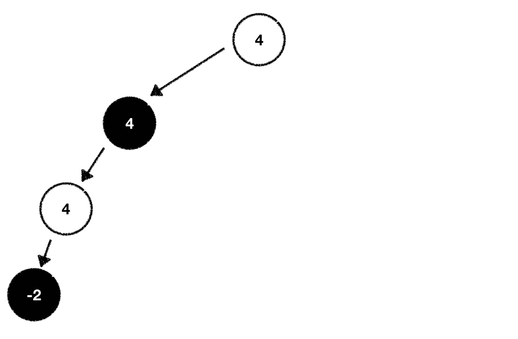
While walking through the potential moves we can play given the current game state we're in we should build our tree in a depth-first fashion. This means that we should start at one node and expand it by playing the game all the way to the end before we back up and pick the next node we want to explore: Following this procedure allows us to identify moves which will never be played early on. After all, one player maximizes the outcome while the other minimizes it. The part of the search tree where a player would end up in a worse situation based on the evaluation function can be entirely removed from the list of nodes we want to expand and explore. We prune those nodes from our search tree and therefore reduce its width. The larger the branching factor of the tree, the higher the amount of computations we can potentially save!

Assuming we can reduce the width by an average of 10 we would end up with $w^d = (30 - 10)^{85} = 20^{85}$ computations we have to perform. That's already a huge win.

This technique of pruning parts of the search tree which will never be considered during gameplay is called Alpha-Beta pruning. Alpha-Beta pruning got its name from the parameters $\alpha$ and $\beta$ which are used to keep track of the best score either player can achieve while walking the tree.

Code

def minimax(state, max_depth, is_player_minimizer, alpha, beta):
    if max_depth == 0 or state.is_end_state():
        return evaluation_function(state)

    if is_player_minimizer:
        value = -math.inf
        for move in state.possible_moves():
            evaluation = minimax(move, max_depth - 1, False, alpha , beta)
            min = min(value, evaluation)
            # Keeping track of our current best score
            beta = min(beta, evaluation)
            if beta <= alpha:
                break
        return value

    value = math.inf
    for move in state.possible_moves():
        evaluation = minimax(move, max_depth - 1, True, alpha, beta)
        max = max(value, evaluation)
        # Keeping track of our current best score
        alpha = max(alpha, evaluation)
        if beta <= alpha:
            break
    return value

Using Alpha-Beta pruning to reduce the trees width helps us utilize the Minimax algorithm in games with large branching factors which were previously considered as computationally too expensive.

In fact Deep Blue, the Chess computer developed by IBM which defeated the Chess world champion Garry Kasparov in 1997 heavily utilized parallelized Alpha-Beta based search algorithms.

Monte Carlo Tree Search

It seems like Minimax combined with Alpha-Beta pruning is enough to build sophisticated game AIs. But there's one major problem which can render such techniques useless. It's the problem of defining a robust and reasonable evaluation function. Recall that in Chess our evaluation function added up all the white pieces on the board and subtracted all the black ones. This resulted in high values when white had an edge and in low values when the situation was favorable for black. While this function is a good baseline and is definitely worthwhile to experiment with there are usually more complexities and subtleties one needs to incorporate to come up with a sound evaluation function.

Simple evaluation metrics are easy to fool and exploit once the underlying internals are surfaced. This is especially true for more complex games such as Go. Engineering an evaluation function which is complex enough to capture the majority of the necessary game information requires a lot of thought and interdisciplinary domain expertise in Software Engineering, Math, Psychology and the game at hand.

Isn't there a universally applicable evaluation function we could leverage for all games, no matter how simple or complex they are?

Yes, there is! And it's called randomness. With randomness we let chance be our guide to figure out which next move might be the best one to pick.

In the following we'll explore the so-called Monte Carlo Tree Search (MCTS) algorithm which heavily relies on randomness (the name "Monte Carlo" stems from the gambling district in Monte Carlo) as a core component for value approximations.

As the name implies, MCTS also builds up a game tree and does computations on it to find the path of the highest potential outcome. But there's a slight difference in how this tree is constructed.

Let's once again pretend that we're playing Chess as player white. We've already played for a couple of rounds and it's on us again to pick the next move we'd like to play. Additionally let's pretend that we're not aware of any evaluation function we could leverage to compute the value of each possible move. Is there any way we could still figure out which move might put us into a position where we could win at the end?

As it turns out there's a really simple approach we can take to figure this out. Why don't we let both player play dozens of random games starting from the state we're currently in? While this might sound counterintuitive it make sense if you think about it. If both player start in the given game state, play thousands of random games and player white wins 80% of the time, then there must be something about the state which gives white an advantage. What we're doing here is basically exploiting the Law of large numbers (LLN) to find the "true" game outcome for every potential move we can play.

The following description will outline how the MCTS algorithm works in detail. For the sake of simplicity we again focus solely on 2 playable moves in any given state (as we've already discovered there are on average ~30 different moves we can play in Chess).

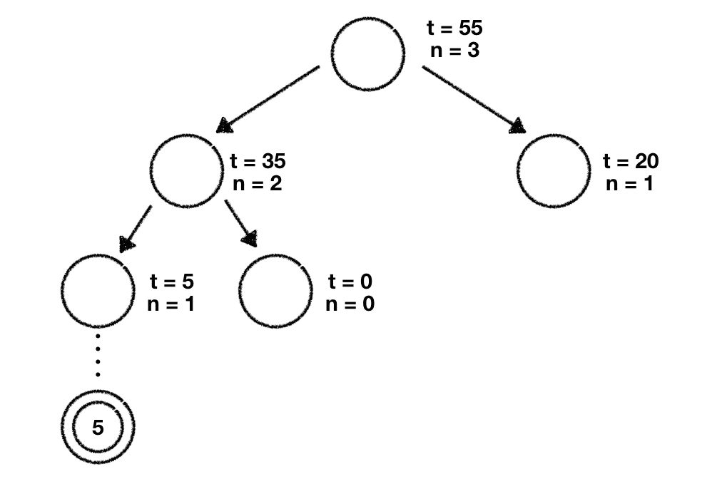
Before we move on we need to get some minor definitions out of the way. In MCTS we keep track of 2 different parameters for every single node in our tree. We call those parameters $t$ and $n$. $t$ stands for "total" and represents the total value of that node. $n$ is the "number of visits" which reflects the number of times we've visited this node while walking through the tree. When creating a new node we always initialize both parameters with the value 0.

In addition to the 2 new parameters we store for each node, there's the so-called "Upper Confidence Bound 1" (UCT) formula which looks like this

This formula basically helps us in deciding which upcoming node and therefore potential game move we should pick to start our random game series (called "rollout") from. In the formula $x_i$ represents the average value of the game state we're working with, $C$ is a constant called "temperature" we need to define manually (we just set it to 1.5 in our example here. More on that later), $N$ represents the parent node visits and $n_i$ represents the current nodes visits. When using this formula on candidate nodes to decide which one to explore further, we're always interested in the largest result.

Don't be intimidated by the Math and just note that this formula exists and will be useful for us while working with out tree. We'll get into more details about the usage of it while walking through our tree.

With this out of the way it's time apply MCTS to find the best move we can play.

We start with the same root node of the tree we're already familiar with. This root node is our start point and reflects the current game state. Based on this node we branch off our 2 child nodes: 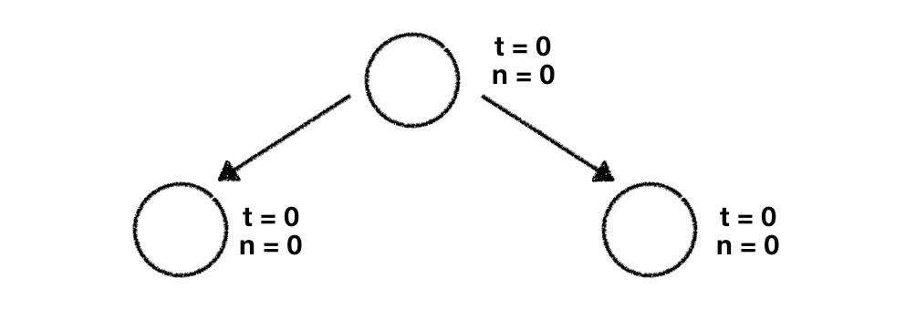The first thing we need to do is to use the UCT formula from above and compute the results for both child nodes. As it turns out we need to plug in 0 for almost every single variable in our UCT formula since we haven't done anything with our tree and its nodes yet. This will result in $\infty$ for both calculations.

We've replaced the 0 in the denominator with a very small number because division by zero is not defined

Given this we're free to choose which node we want to explore further. We go ahead with the leftmost node and perform our rollout phase which means that we play dozens of random games starting with this game state.

Once done we get a result for this specific rollout (in our case the percentage of wins for player white). The next thing we need to do is to propagate this result up the tree until we reach the root node. While doing this we update both $t$ and $n$ with the respective values for every node we encounter. Once done our tree looks like this: 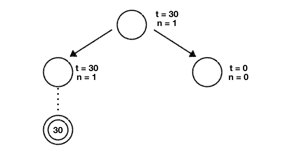Next up we start at our root node again. Once again we use the UCT formula, plug in our numbers and compute its score for both nodes:

Given that we always pick the node with the highest value we'll now explore the rightmost one. Once again we perform our rollout based on the move this node proposes and collect the end result after we've finished all our random games.

The last thing we need to do is to propagate this result up until we reach the root of the tree. While doing this we update the parameters of every node we encounter.

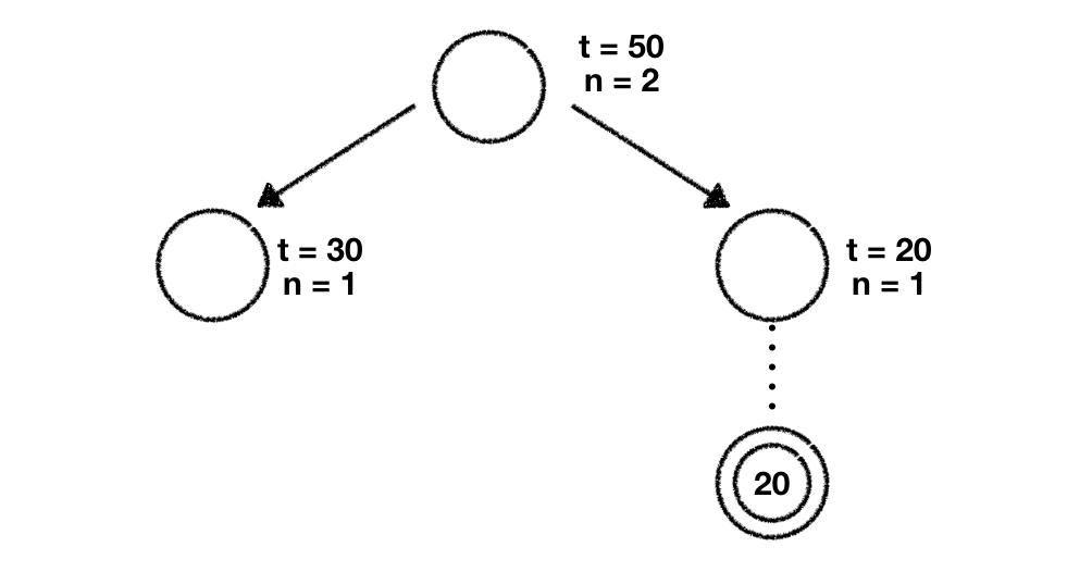
We've now successfully explored 2 child nodes in our tree. You might've guessed it already. We'll start again at our root node and calculate every child nodes UCT score to determine the node we should further explore. In doing this we get the following values:

The largest value is the one we've computed for the leftmost node so we decide to explore that node further.

Given that this node has no child nodes we add two new nodes which represent the potential moves we can play to the tree. We initialize both of their parameters ($t$ and $n$) with 0.

Now we need to decide which one of those two nodes we should explore further. And you're right. We use the UCT formula to calculate their values. Given that both have $t$ and $n$ values of zero they're both $\infty$ so we decide to pick the leftmost node. Once again we do a rollout, retrieve the value of those games and propagate this value up to the tree until we reach the trees root node, updating all the node parameters along the way.

The next iteration will once again start at the root node where we use the UCT formula to decide which child node we want to explore further. Since we can see a pattern here and I don't want to bore you I'm not going to describe the upcoming steps in great detail. What we'll be doing is following the exact same procedure we've used above which can be summarized as follows:

1. Start at the root node and use the UCT formula to calculate the score for every child node

2. Pick the child node for which you've computed the highest UCT score

3. Check if the child has already been visited

   • If not, do a rollout
   • If yes, determine the potential next states from there
   • Use the UCT formula to decide which child node to pick
   • Do a rollout

4. Propagate the result back through the tree until you reach the root node

We iterate over this algorithm until we run out of time or reached a predefined threshold value of visits, depth or iterations. Once this happens we evaluate the current state of our tree and pick the child node(s) which maximize the value $t$. Thanks to dozens of games we've played and the Law of large numbers we can be very certain this move is the best one we can possibly play.

That's all there is. We've just learned, applied and understood Monte Carlo Tree Search!

You might agree that it seems like MCTS is very compute intensive since you have to run through thousands of random games. This is definitely true and we need to be very clever as to where we should invest our resources to find the most promising path in our tree. We can control this behavior with the aforementioned "temperature" parameter $C$ in our UCT formula. With this parameter we balance the trade-off between "exploration vs. exploitation".

A large $C$ value puts us into "exploration" mode. We'll spend more time visiting least-explored nodes. A small value for $C$ puts us into "exploitation" mode where we'll revisit already explored nodes to gather more information about them.

Given the simplicity and applicability due to the exploitation of randomness, MCTS is a widely used game tree search algorithm. DeepMind extended MCTS with Deep Neural Networks to optimize its performance in finding the best Go moves to play. The resulting Game AI was so strong that it reached superhuman level performance and defeated the Go World Champion Lee Sedol 4-1.

Conclusion

In this blog post we've looked into 2 different tree search algorithms which can be used to build sophisticated Game AIs.

While Minimax combined with Alpha-Beta pruning is a solid solution to approach games where an evaluation function to estimate the game outcome can easily be defined, Monte Carlo Tree Search (MCTS) is a universally applicable solution given that no evaluation function is necessary due to its reliance on randomness.

Raw Minimax and MCTS are only the start and can easily be extended and modified to work in more complex environments. DeepMind cleverly combined MCTS with Deep Neural Networks to predict Go game moves whereas IBMextended Alpha-Beta tree search to compute the best possible Chess moves to play.

Do you have any questions, feedback or comments? Feel free to reach out via E-Mail or connect with me on Twitter.

Additional Resources

Do you want to learn more about Minimax and Monte Carlo Tree Search? The following list is a compilation of resources I found useful while studying such concepts.

If you're really into modern Game AIs I highly recommend the book "Deep Learning and the Game of Go" by Max Pumperla and Kevin Ferguson. In this book you'll implement a Go game engine and refine it step-by-step until at the end you implement the concepts DeepMind used to build AlphaGo and AlphaGo Zero based on their published research papers.

• Wikipedia - Minimax
• Wikipedia - Alpha-Beta Pruning
• Wikipedia - Expectiminimax
• MIT OpenCourseWare - Games, Minimax, and Alpha-Beta
• Sebastian Lague - Minimax and alpha-beta pruning
• Wikipedia - Monte Carlo Tree Search
• John Levine - Monte Carlo Tree Search