Logistic Regression from scratch


You can find working code examples (including this one) in my lab repository on GitHub.
Sometimes it's necessary to split existing data into several classes in order to predict new, unseen data. This problem is called classification and one of the algorithms which can be used to learn those classes from data is called Logistic Regression.
In this article we'll take a deep dive into the Logistic Regression model to learn how it differs from other regression models such as Linear- or Multiple Linear Regression, how to think about it from an intuitive perspective and how we can translate our learnings into code while implementing it from scratch.
Linear Regression vs. Logistic Regression
If you've read the post about Linear- and Multiple Linear Regression you might remember that the main objective of our algorithm was to find a best fitting line or hyperplane respectively.
To recap real quick, a line can be represented via the slop-intercept form as follows:
Here, represents the slope and the y-intercept.
In Linear Regression we've used the existing data to find a line in slope-intercept form (a and combination) which "best-fitted through" such data.
Extending the slope-intercept form slightly to support multiple values and multiple slopes (we'll use instead of ) yields the following:
This "scaled-up" slope-intercept formula was used in the Multiple Linear Regression model to find the and values for the hyperplane which "best-fitted" the data. Once found we were able to use it for predictions by plugging in values to get respective values.
Linear Regression models always map a set of values to a resulting value on a continuous scale. This means that the value can e.g. be , or . How would we use such a Regression model if our value is categorical such as a binary value which is either or ? Is there a way to define a threshold so that a value such as is assigned to the category while a small value such as gets assigned to the category ?
That's where Logistic Regression comes into play. With Logistic Regression we can map any resulting value, no matter its magnitude to a value between and .
Let's take a closer look into the modifications we need to make to turn a Linear Regression model into a Logistic Regression model.
Sigmoid functions
At the very heart of Logistic Regression is the so-called Sigmoid function. A Sigmoid function is a class of functions which follows an S-shape when plotted.
The most prominent Sigmoid function is the so-called Logistic function which was developed by Pierre Francois Verhulst to model population grown. It's mathematically described via this formula:
Don't be intimidated by the math! Right now all you need to know is that this function takes any value and maps it to a value which ranges from to .
Plotting the function for a range of values proofs this claim and results in the aforementioned S-shape curve:
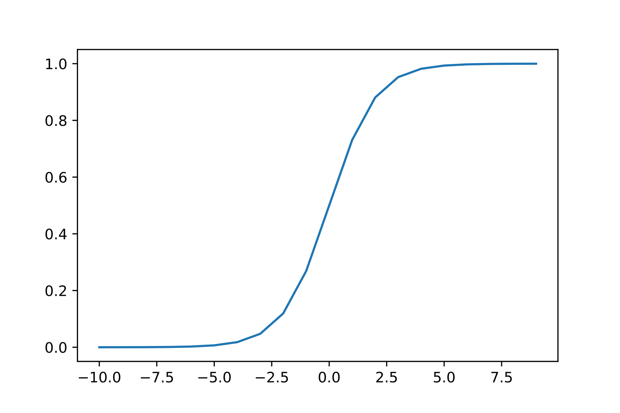
Note that the function gets closer and closer to the value or as the values get smaller or larger respectively. Also note that the value results in the value .
This is exactly what we need. with this function we're able to "squish" any number, no matter its magnitude into a value ranging from to . This makes the function outcome predictable which is useful when we later on define threshold values to associate function outputs with classes.
Let's turn the function into code:
def sigmoid(x: float) -> float:
    return 1 / (1 + exp(-x))

assert sigmoid(0) == 0.5
Note: Although there are many different Sigmoid functions to choose from, a lot of people use the name "Sigmoid function" when talking about the Logistic function. We'll adhere to this convention and use the term "Sigmoid function" as a synonym for Logistic function.
From Linear Regression to Logistic Regression
Now that we've learned about the "mapping" capabilities of the Sigmoid function we should be able to "wrap" a Linear Regression model such as Multiple Linear Regression inside of it to turn the regressions raw output into a value ranging from to .
Let's translate this idea into Math. Recall that our Multiple Linear Regression model looks like this:
"Wrapping" this in the Sigmoid function (we use to represent the Sigmoid function) results in the following:
Easy enough! Let's turn that into code.
The first thing we need to do is to implement the underlying Multiple Linear Regression model. Looking at the Math it seems to be possible to use the dot-product to calculate the and part to which we then add the single value.
To make everything easier to calculate and implement we'll use a small trick. Multiplying a value by the identify yields the value so we prepend to the values and to the values. This way we can solely use the dot-product calculation without the necessity to add separately later on. Here's the mathematical formulation of that trick:
Once we've calculated the dot-product we need to pass it into the Sigmoid function such that its result is translated ("squished") into a value between and .
Here's the implementation for the dot function which calculates the dot-product:
def dot(a: List[float], b: List[float]) -> float:
    assert len(a) == len(b)
    return sum([a_i * b_i for a_i, b_i in zip(a, b)])

assert dot([1, 2, 3, 4], [5, 6, 7, 8]) == 70
And here's the squish function which takes as parameters the and values (remember that we've prepended a to the values and the to the values), uses the dot function to calculate the dot-product of and and then passes this result into the Sigmoid function to map it to a value between and :
def squish(beta: List[float], x: List[float]) -> float:
    assert len(beta) == len(x)
    # Calculate the dot product
    dot_result: float = dot(beta, x)
    # Use sigmoid to get a result between 0 and 1
    return sigmoid(dot_result)

assert squish([1, 2, 3, 4], [5, 6, 7, 8]) == 1.0
The intuition behind the 0-1 range
We've talked quite a lot about how the Sigmoid function is our solution to make the function outcome predictable as all values are mapped to a - range. But what does a value in that range represent? Let's take a look at an example.
The following is a data set which describes how long students have studied for an exam and whether they've passed the exam given the hours they've studied.
| Hours studied | Exam Passed |
|---|---|
| 0,5 | 0 |
| 1,0 | 0 |
| 1,5 | 0 |
| 2,0 | 0 |
| 2,5 | 1 |
| 3,0 | 0 |
| 3,5 | 1 |
| 4,0 | 1 |
| 4,5 | 0 |
| 5,0 | 1 |
| 5,5 | 1 |
| 6,0 | 1 |
Taking a glance at the data it seems to be that the more hours the students studied, the more likely they were to pass the exam. Intuitively that makes sense.
Let's plot the data to ensure that our intuition is correct:
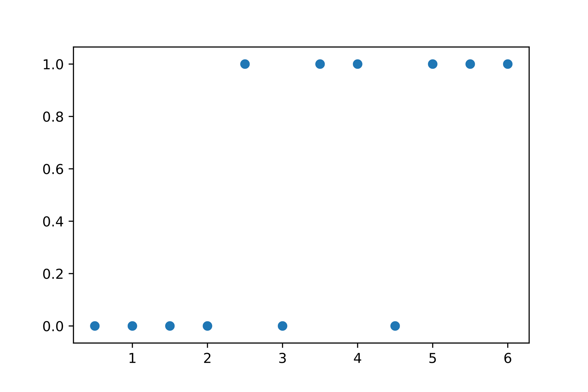
Looking at the plotted data we can immediately see that the values seem to "stick" to either the bottom or top of the graph. Given that it seems to be infeasible to use a Linear Regression model to find a line which best describes the data. How would this line be fitted through the data if the values we'd expect this line should produce are either or ?
Let's try a thought experiment. What would happen if we've somehow found some coefficients for the Linear Regression model which "best" describe the data and pass the result it computes through the Sigmoid function? Here's the graph from above with the Sigmoid function added to it:
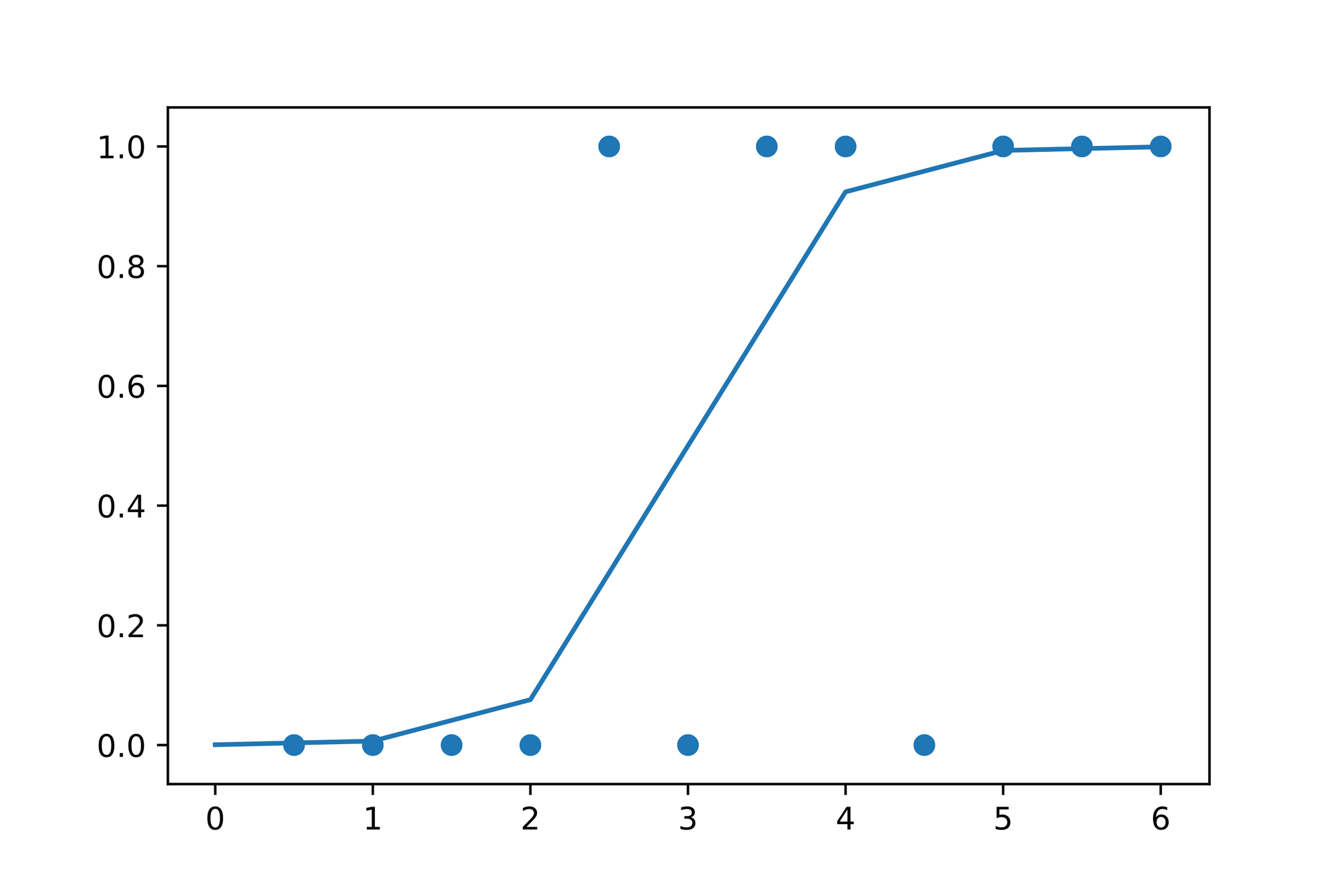
Looking at the plotting above we can see that the Sigmoid function ensures that the result from the "underlying" Linear Regression model is mapped onto a scale between and , which in turn makes it possible to e.g. define a threshold at to say that a value which is greater than might be a predictor for a student passing the exam while a value less than might mean that she'll fail the exam.
Note that the wording in the last sentence isn't a coincidence. The value the Sigmoid function produces can be interpreted as a probability where means probability and means a probability.
The Probability Density Function
As it turns out we can translate our findings from the previous section into a function called Probability density function or (PDF for short).
In particular we can define a conditional probability which states that given some and , each corresponding should equal with probability and with probability :
Looking at the formula above it might be a mystery how we deduced it from our verbal description from above. Here's something I want you to try: Please apply the formula by setting to and after that to and see what happens. What you'll notice is that depending on what value you set to, only one part of the formula stays the same while the other is canceled out.
Here's what we'll end up with if we set to and :
And that's exactly the desired behavior we described above.
Deriving a Loss function
With Logistic Regression our main objective is to find the models parameters which maximize the likelihood that for a pair of values the value our model calculates is as close to the actual value as possible.
In order to find the optimal parameters we need to somehow calculate how "wrong" our models predictions are with the current setup.
In the previous section we talked about the Probability Density Function (PDF) which seems to capture exactly that. We just need to tweak this function slightly so that it's easier for us to do calculations with it later on.
The main tweak we'll apply is that we "wrap" our individual PDF calculations for and in the function. The Logarithm has the nice property that it's strictly increasing which makes it easier to do calculations on its data later on. Furthermore our PDFs main property is still preserved since any set of values that maximizes the likelihood of predicting the correct also maximizes the likelihood.
Here are the PDFs two major parts "wrapped" in the function:
There's only one minor issue we need to resolve. Overall we're attempting to minimize the amount of wrong predictions our model produces, but looking at the graph of the Logarithm once again we see that the function is strictly increasing. We "mirror" the logarithm at the axis ("turning" it upside down) by multiplying it with . Hence our two functions now look like this:
Now the last thing we want to do here is to put both functions back together into one equation like we did with our composite PDF function above. Doing this results in the following:
This function is called Logarithmic Loss (or Log Loss / Log Likelihood) and it's what we'll use later on to determine how "off" our model is with its prediction. Again, you might want to set to or to see that one part of the equation is canceled out.
Let's turn that into code:
def neg_log_likelihood(y: float, y_pred: float) -> float:
    return -((y * log(y_pred)) + ((1 - y) * log(1 - y_pred)))

assert 2.30 < neg_log_likelihood(1, 0.1) < 2.31
assert 2.30 < neg_log_likelihood(0, 0.9) < 2.31
assert 0.10 < neg_log_likelihood(1, 0.9) < 0.11
assert 0.10 < neg_log_likelihood(0, 0.1) < 0.11
Next up let's use our codified version of Log Loss to create plots for and :
xs_nll: List[float] = [x / 10000 for x in range(1, 10000)]

fig, (ax1, ax2) = plt.subplots(1, 2)
ax1.plot(xs_nll, [neg_log_likelihood(1, x) for x in xs_nll])
ax1.set_title('y = 1')
ax2.plot(xs_nll, [neg_log_likelihood(0, x) for x in xs_nll])
ax2.set_title('y = 0');
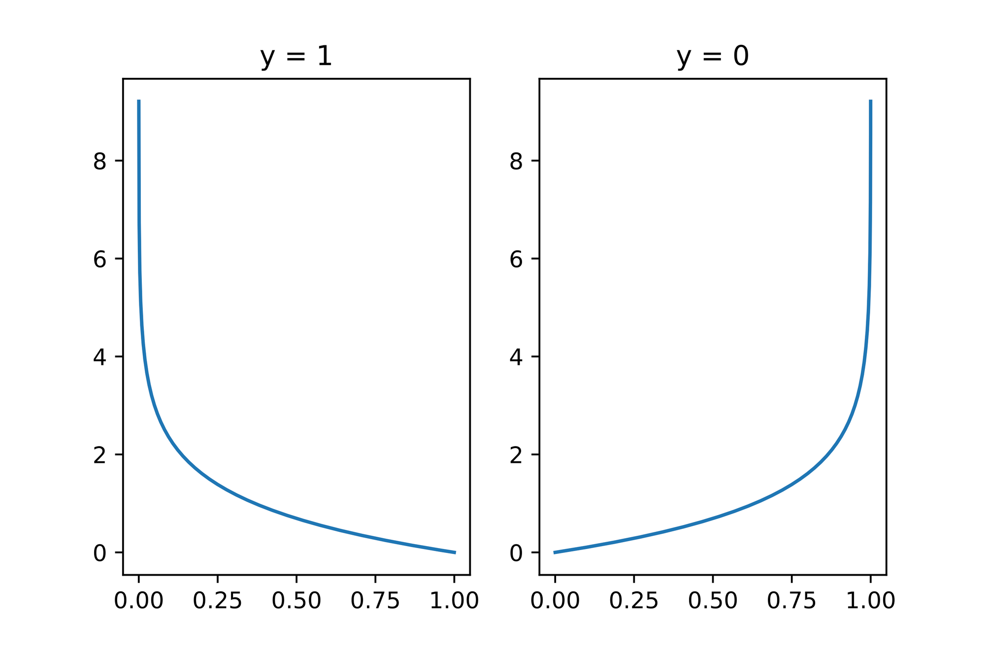
As we can see, the more wrong the prediction, the higher the calculated error. The Log Loss function therefore "punished" wrongdoing more than it rewards "rightdoing".
To calculate the overall error of our whole data set we sum up each individual Log Loss calculation and average it:
Here's the codified version:
def error(ys: List[float], ys_pred: List[float]) -> float:
    assert len(ys) == len(ys_pred)
    num_items: int = len(ys)
    sum_nll: float = sum([neg_log_likelihood(y, y_pred) for y, y_pred in zip(ys, ys_pred)])
    return (1 / num_items) * sum_nll

assert 2.30 < error([1], [0.1]) < 2.31
assert 2.30 < error([0], [0.9]) < 2.31
assert 0.10 < error([1], [0.9]) < 0.11
assert 0.10 < error([0], [0.1]) < 0.11
Optimizing via Gradient Descent
Now the last missing piece we need to implement is the optimization step. What we want at the end of the day is a Logistic Regression model with the parameters which in combination with values produce the most accurate prediction for any value.
Given that we can now calculate the error our current model with its parameters produces we can iteratively change the parameters until we reach a point where our model cannot improve (can't reduce the error value) anymore.
The algorithm which implements exactly that is called Gradient Descent.
Note: I already wrote a dedicated post explaining the algorithm in great detail so I won't go into too much detail here and would encourage you to read the article if you're unfamiliar with Gradient Descent.
The gist of it is that given our Log Loss function we can find a set of parameters for which the error the Log Loss function calculates is the smallest. We've therefore found a local (or global) minimum if the error cannot be reduced anymore. To figure out "where" the minimum is located we'll use the error functions gradient which is a vector and guides us to that position.
Since we repeat such calculations over and over again we're iteratively descending down the error functions surface, hence the name Gradient Descent.
Calculating the gradient is done by computing the partial derivatives of the Log Loss function with respect to the individual values in our vector.
Here's the mathematical representation:
And here's the implementation in code:
grad: List[float] = [0 for _ in range(len(beta))]
for x, y in zip(xs, ys):
    err: float = squish(beta, x) - y
    for i, x_i in enumerate(x):
        grad[i] += (err * x_i)
grad = [1 / len(x) * g_i for g_i in grad]
Again, if you're unfamiliar with gradients and partial derivatives you might want to read my article about the Gradient Descent algorithm.
We finally got all the pieces in place! Let's grab some data and use the Logistic Regression model to classify it!
Putting it into practice
The data set we'll be using is similar to what we've already seen in our example above where we tried to predict whether a student will pass an exam based on the hours she studied.
You can download the data set here. Inspecting the data we can see that there are 2 floating point values and an integer value which represents the label and (presumably) indicates whether the student in question has passed or failed the exam.
Our task is it to use this data set to train a Logistic Regression model which will help us assign the label or (i.e. classify) new, unseen data points.
The first thing we need to do is to download the .txt file:
wget -nc -P data https://raw.githubusercontent.com/animesh-agarwal/Machine-Learning/5b2d8a71984016ae021094641a3815d6ea9ac527/LogisticRegression/data/marks.txtNext up we need to parse the file and extract the and values:
marks_data_path: Path = data_dir / 'marks.txt'

xs: List[List[float]] = []
ys: List[float] = []

with open(marks_data_path) as file:
    for line in file:
        data_point: List[str] = line.strip().split(',')
        x1: float = float(data_point[0])
        x2: float = float(data_point[1])
        y: int = int(data_point[2])
        xs.append([x1, x2])
        ys.append(y)
It's always a good idea to plot the data to see if there are any outliers or other surprises we have to deal with:
x1s: List[float] = [x[0] for x in xs]
x2s: List[float] = [x[1] for x in xs]

plt.scatter(x1s, x2s, c=ys)
plt.axis([min(x1s), max(x1s), min(x2s), max(x2s)]);
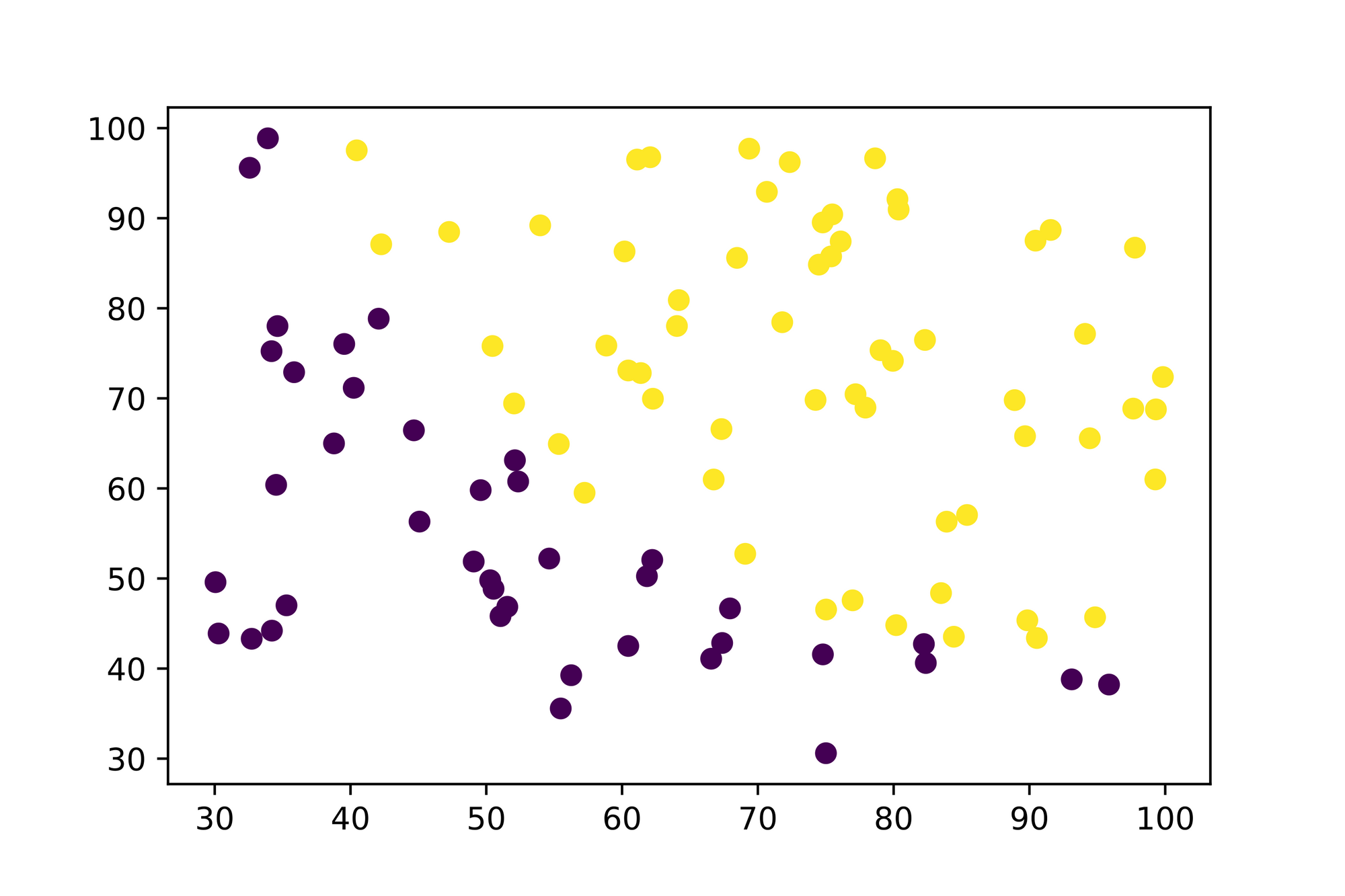
Looks like we're (almost) good here. There's only one aspect we need to further inspect. If you're looking at the axes you see that the values are ranging from to . Working with such large values can result into problems when working with and later on. We'll resolve this problem in a minute.
You might recall from the beginning of the post that we applied a trick where we prepend every vector with a and prepend the to the vector in order to make it possible to use the dot-product (which is a simpler calculation).
The following code prepends a to every vector so that we can leverage the computation trick later on:
for x in xs:
    x.insert(0, 1)

xs[:5]

# [[1, 34.62365962451697, 78.0246928153624],
# [1, 30.28671076822607, 43.89499752400101],
# [1, 35.84740876993872, 72.90219802708364],
# [1, 60.18259938620976, 86.30855209546826],
# [1, 79.0327360507101, 75.3443764369103]]
Next up we'll tackle the scaling problem we've touched upon in the paragraph above. What we'll do to resolve this problem is to standardize (often done via the "z-score") the whole data set:
xs = z_score(xs)

xs[:5]

# [[1, -1.5942162646576388, 0.6351413941754435],
# [1, -1.8171014180340745, -1.2014885239142388],
# [1, -1.531325157335502, 0.3594832875590465],
# [1, -0.28068723821760927, 1.0809228071415948],
# [1, 0.6880619310375534, 0.4909048515228952]]
If you're curious what the z_score function does check out the whole implementation in my lab repository on GitHub.
And now we're finally in a position where we can train our Logistic Regression Model via Gradient Descent. We'll start with some random guesses for our models parameters and iteratively optimize our model by computing its current overall "wrongdoing" with the error function and then using the error functions gradient to update the value to yield a smaller error in the next iteration. Eventually we'll converge to a local minimum which results in values computing the smallest error.
beta: List[float] = [random() / 10 for _ in range(3)]

print(f'Starting with "beta": {beta}')

epochs: int = 5000
learning_rate: float = 0.01

for epoch in range(epochs):
    # Calculate the "predictions" (squishified dot product of `beta` and `x`) based on our current `beta` vector
    ys_pred: List[float] = [squish(beta, x) for x in xs]

    # Calculate and print the error
    if epoch % 1000 == True:
        loss: float = error(ys, ys_pred)
        print(f'Epoch {epoch} --> loss: {loss}')

    # Calculate the gradient
    grad: List[float] = [0 for _ in range(len(beta))]
    for x, y in zip(xs, ys):
        err: float = squish(beta, x) - y
        for i, x_i in enumerate(x):
            grad[i] += (err * x_i)
    grad = [1 / len(x) * g_i for g_i in grad]

    # Take a small step in the direction of greatest decrease
    beta = [b + (gb * -learning_rate) for b, gb in zip(beta, grad)]

print(f'Best estimate for "beta": {beta}')

# Starting with "beta": [0.06879018957747185, 0.060750489548129484, 0.08122488791609535]
# Epoch 1 --> loss: 0.6091560801945126
# Epoch 1001 --> loss: 0.2037432848849053
# Epoch 2001 --> loss: 0.20350230881468107
# Epoch 3001 --> loss: 0.20349779972872906
# Epoch 4001 --> loss: 0.20349770371660023
# Best estimate for "beta": [1.7184091311489376, 4.01281584290694, 3.7438191715393083]
Now that our model is trained we can calculate some statistics to see how accurate it is. For these calculations we'll set the threshold to which means that every value above our model produces is considered a and every value which is less than is considered to be a .
total: int = len(ys)
thresh: float = 0.5
true_positives: int = 0
true_negatives: int = 0
false_positives: int = 0
false_negatives: int = 0

for i, x in enumerate(xs):
    y: int = ys[i]
    pred: float = squish(beta, x)
    y_pred: int = 1
    if pred < thresh:
        y_pred = 0
    if y == 1 and y_pred == 1:
        true_positives += 1
    elif y == 0 and y_pred == 0:
        true_negatives += 1
    elif y == 1 and y_pred == 0:
        false_negatives += 1
    elif y == 0 and y_pred == 1:
        false_positives += 1

print(f'True Positives: {true_positives}')
print(f'True Negatives: {true_negatives}')
print(f'False Positives: {false_positives}')
print(f'False Negatives: {false_negatives}')
print(f'Accuracy: {(true_positives + true_negatives) / total}')
print(f'Error rate: {(false_positives + false_negatives) / total}')

# True Positives: 55
# True Negatives: 34
# False Positives: 6
# False Negatives: 5
# Accuracy: 0.89
# Error rate: 0.11
Finally let's plot the decision boundary so that we can see where our model "draws the line":
x1s: List[float] = [x[1] for x in xs]
x2s: List[float] = [x[2] for x in xs]
plt.scatter(x1s, x2s, c=ys)
plt.axis([min(x1s), max(x1s), min(x2s), max(x2s)]);

m: float = -(beta[1] / beta[2])
b: float = -(beta[0] / beta[2])

x2s: List[float] = [m * x[1] + b for x in xs]

plt.plot(x1s, x2s, '--');
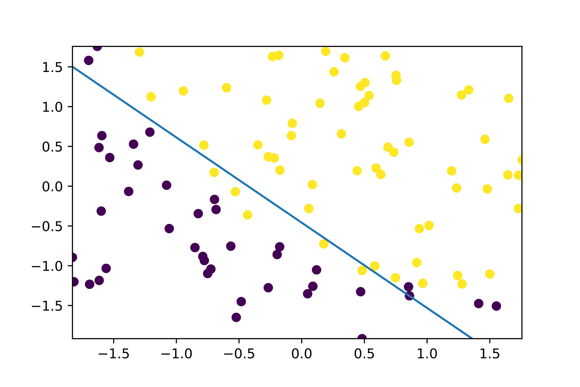
Great! Looks like our model correctly learned how to classify new, unseen data as it considers everything "above" and "below" the decision boundary as a separate class which seems to be in alignment with the data points from our data set!
Conclusion
In some situations it's a requirement to classify new, unseen data. Logistic Regression is a powerful Machine Learning model which makes it possible to learn such classifications based on existing data.
In this blog post we took a deep dive into Logistic Regression and all its moving parts. We've learned about Sigmoid functions and how they can be used in conjunction with a Linear Regression model to project values of arbitrary magnitude onto a scale between and which is exactly what we need when we want to do binary classification.
Once we understood the mathematics and implemented the formulas in code we took an example data set and applied our Logistic Regression model to a binary classification problem. After training our model we were able to draw the decision boundary it learned to visually validate that it correctly learned how to separate the data into two (binary) subsets.
Do you have any questions, feedback or comments? Feel free to reach out via E-Mail or connect with me on Twitter.
Additional Resources
The following is a list of resources I've used to write this article. Other, useful resources are linked within the article itself: