Gradient Descent from scratch

Philipp Muens

Philipp Muens

You can find working code examples (including this one) in my lab repository on GitHub.

Gradient Descent is one of the most fundamental optimization techniques used in Machine Learning. But what is a gradient? On what do we descent down and what do we even optimize in the first place?

Those might be some of the questions which come to mind when having the first encounters with Gradient Descent. Let's answer those questions while implementing the Gradient Descent optimization technique from scratch.

Optimizations and loss functions

Many Machine Learning problems require some form of optimization. Usually the algorithm starts with an initial guess as to what the correct answer might be and then slowly adapts its parameters to be less wrong with every consecutive trial.

This learning process through trial and error repeats until the algorithm has learned to "correctly" predict the results for the training- and test data it gets fed.

In order to figure out how wrong our algorithm is with its predictions, we need to define the notion of a loss function. The loss function compares the guesses and the actual values and turns the differences between the two into a measurement we can use to quantify the quality of our algorithm. Prominent loss function are Mean squared error (MSE), Root mean square error (RMSE) or Sum of squared errors (SSE).

Imagine that we're plotting the loss (i.e. "wrongdoing") the algorithm produces as a surface in a multi dimensional space (such as 3D). Intuitively it seems to make sense to find the "place" on this surface where the algorithm is doing the fewest mistakes. That's exactly where Gradient Descent comes into play. With Gradient Descent we take a "walk" on this surface to find such a place.

Gradient Descent by example

As we've already discovered, loss functions and optimizations are usually intertwined when working on Machine Learning problems. While it makes sense to teach them together I personally believe that it's more valuable to keep things simple and focused while exploring core ideas. Therefore for the rest of this post we'll solely focus on Gradient Descent as a mathematical optimization technique which can be applied in a variety of different domains (including Machine Learning problems).

A Paraboloid

The first thing we should do is to define the function we want to run the Gradient Descent algorithm on. Most examples explain the algorithms core concepts with a single variable function such as a function drawn from the class of parabolas (e.g. $x^2$ ). Single variable functions can be easily plotted in a 2 dimensional space along the $x$ and $y$ axes. Besides other nice properties, dealing with only 2 dimensions makes the involved math a whole lot easier. Real world Machine Learning problems however deal with data in an order of magnitude higher dimensions. While there's a slightly steeper learning curve to go from 2D to 3D there's pretty much nothing new to learn to go from 3D to $n$ D. Because of that we'll apply Gradient Descent to a multivariable function with 2 variables.

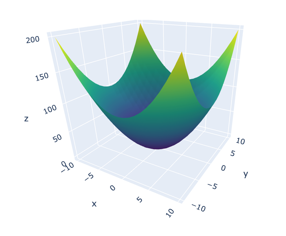
Most of us studied the properties of quadratic functions via parabolas in school. But is there an equivalent function which can be plotted in 3 dimensions? Imagine that you have a parabola and spin it like a centrifuge along its $y$ -axis. What you'd end up with is a surface called a paraboloid, a "3 dimensional parabola".

There are various ways to define paraboloids but in our case let's use the "infinite paraboloid" which is defined as follows:

x^2 + y^2

Translating the math into code results in:

def paraboloid(x: float, y: float) -> float:
    return x ** 2 + y ** 2

Simple enough. Next up we should generate some test data, pass it into our paraboloid function and plot the results to see if everything works as expected:

# Test data generation (only really necessary for the plotting below)
xs_start = ys_start = -10
xs_stop = ys_stop = 11
xs_step = ys_step = 1

xs: List[float] = [i for i in range(xs_start, xs_stop, xs_step)]
ys: List[float] = [i for i in range(ys_start, ys_stop, ys_step)]
zs: List[List[float]] = []

for x in xs:
    temp_res: List[float] = []
    for y in ys:
        result: float = paraboloid(x, y)
        temp_res.append(result)
    zs.append(temp_res)

print(f'xs: {xs}\n')
# xs: [-10, -9, -8, -7, -6, -5, -4, -3, -2, -1, 0, 1, 2, 3, 4, 5, 6, 7, 8, 9, 10]

print(f'ys: {ys}\n')
# ys: [-10, -9, -8, -7, -6, -5, -4, -3, -2, -1, 0, 1, 2, 3, 4, 5, 6, 7, 8, 9, 10]

print(f'zs: {zs[:5]} ...\n')
# zs: [[200, 181, 164, 149, 136, 125, 116, 109, 104, 101, 100, 101, 104, 109, 116, 125, 136, 149, 164, 181, 200], [181, 162, 145, 130, 117, 106, 97, 90, 85, 82, 81, 82, 85, 90, 97, 106, 117, 130, 145, 162, 181], [164, 145, 128, 113, 100, 89, 80, 73, 68, 65, 64, 65, 68, 73, 80, 89, 100, 113, 128, 145, 164], [149, 130, 113, 98, 85, 74, 65, 58, 53, 50, 49, 50, 53, 58, 65, 74, 85, 98, 113, 130, 149], [136, 117, 100, 85, 72, 61, 52, 45, 40, 37, 36, 37, 40, 45, 52, 61, 72, 85, 100, 117, 136]] ...

Plotting the graph (using the Plotly library) can be done with the following code:

fig = go.Figure(go.Surface(x=xs, y=ys, z=zs, colorscale='Viridis'))
fig.show()

Paraboloid

Gradients and derivatives

According to Wikipedia the definition of a gradient is:

... a vector-valued function $f$ ..., whose value at a point $p$ is the vector whose components are the partial derivatives of $f$ at $p$ .

I agree that this sounds overwhelming but the core concepts of a gradient are really simple. What this quote from above tries to convey is that for any given point $p$ on the functions plotted surface there's a vector consisting of partial derivatives which points in the direction of greatest increase.

With that explanation the only concept we need to sort out is the notion of partial derivatives.

If you've studied Differential Calculus you surely came across the topic of derivatives. To recap real quick, a derivative measures the sensitivity to change of a functions output with respect to changes in its inputs.

Derivatives can be of different orders. One of the most prominent derivatives you surely came across is the first-order derivative which is the slope of a tangent line that tells us whether the function is increasing or decreasing at any given point.

The process of differentiation obeys several rules, some of which we'll apply when walking through the example below to refresh our fond memories of Calculus I.

Let's calculate the first-, second- and third-order derivative of the following function:

x^3 + 2x^2 - 5

According to the differentiation rules, the first-order derivative is:

\frac{d}{dx}(x^3 + 2x^2 - 5) = 3x^2 + 4x

The second-order derivative is:

\frac{d}{dx}(3x^2 + 4x) = 6x + 4

And finally the third-order derivative is:

\frac{d}{dx}(6x + 4) = 6

Why did we do this? As you might recall from above, a gradient is a vector of partial derivatives of function $f$ at point $p$ . So in order to compute gradients we need to compute the partial derivatives of our function $f$ .

We certainly do know how to compute derivatives as we've shown above, but how do we calculate partial derivatives? As it turns out you already know how to calculate partial derivatives if you know how to calculate derivatives. The twist with partial derivatives is that you're deriving with respect to a variable while treating every other variable as a constant.

Let's apply this rule and compute the partial derivatives of our Paraboloid function $x^2 + y^2$ which we call $f$ :

The first partial derivative we calculate is the derivative of $f$ with respect to $x$ , treating $y$ as a constant:

\frac{\partial}{\partial x}(x^2 + y^2) = 2x

The second partial derivative calculation follows the same pattern, deriving $f$ with respect to $y$ while treating $x$ as a constant:

\frac{\partial}{\partial y}(x^2 + y^2) = 2y

Note: Don't get confused by the notation here. While you'd use $\frac{d}{dx}$ for "normal" derivatives you simply use $\frac{\partial}{\partial x}$ for partial derivatives.

And that's it. With those partial derivatives we're now able to compute any gradient for any point $p$ sitting on the plotted surface of function $f$ . Let's translate our findings into code:

def compute_gradient(vec: List[float]) -> List[float]:
    assert len(vec) == 2
    x: float = vec[0]
    y: float = vec[1]
    return [2 * x, 2 * y]

Descending down the surface

Let's recap what we've accomplished so far. First, we've codified and plotted a function called the "infinite paraboloid" which is used throughout this post to demonstrate the Gradient Descent algorithm. Next up we studied gradients, taking a quick detour into Differential Calculus to refresh our memories about differentiation. Finally we computed the partial derivatives of our paraboloid function.

Translating the prose into a mental image, we have a function $f$ which produces a surface in a 3 dimensional space. Given any point $p$ on that surface we can use the gradient (via its partial derivatives) to find a vector pointing into the direction of greatest increase.

That's great, but we're dealing with an optimization problem and for a lot of such applications it's usually desirable to find a global or local minimum. Right now, the gradient vector is pointing upwards to the direction of greatest increase. We need to turn that vector into the opposite direction so that it points to the direction of greatest decrease.

Linear Algebra taught us that doing that is as simple as multiplying the gradient vector by $-1$ . Another neat Linear Algebra trick is to multiply a vector by a number other than $1$ to change its magnitude (= its length). If we're for example multiplying the gradient vector by $0.25$ we would get a vector which has length $\frac{1}{4}$ of its original length.

We finally have all the building blocks in place to put together the Gradient Descent algorithm which eventually finds the nearest local minimum for any given function.

The algorithm works as follows.

Given a function $f$ we want to run Gradient Descent on:

Get the starting position $p$ (which is represented as a vector) on $f$
Compute the gradient at point $p$
Multiply the gradient by a negative "step size" (usually a value smaller than $1$ )
Compute the next position of $p$ on the surface by adding the rescaled gradient vector to the vector $p$
Repeat step 2 with the new $p$ until convergence

Let's turn that into code. First, we should define a compute_step function which takes as parameters the vector $p$ and a "step size" (we call it learning_rate), and computes the next position of $p$ according to the $f$ functions gradient:

def compute_step(curr_pos: List[float], learning_rate: float) -> List[float]:
    grad: List[float] = compute_gradient(curr_pos)
    grad[0] *= -learning_rate
    grad[1] *= -learning_rate
    next_pos: List[float] = [0, 0]
    next_pos[0] = curr_pos[0] + grad[0]
    next_pos[1] = curr_pos[1] + grad[1]
    return next_pos

Next up we should define a random starting position $p$ :

start_pos: List[float]

# Ensure that we don't start at a minimum (0, 0 in our case)
while True:
    start_x: float = randint(xs_start, xs_stop)
    start_y: float = randint(ys_start, ys_stop)
    if start_x != 0 and start_y != 0:
        start_pos = [start_x, start_y]
        break

print(start_pos)
# [6, -3]

And finally we wrap our compute_step function into a loop to iteratively walk down the surface and eventually reach a local minimum:

epochs: int = 5000
learning_rate: float = 0.001

best_pos: List[float] = start_pos

for i in range(0, epochs):
    next_pos: List[float] = compute_step(best_pos, learning_rate)
    if i % 500 == 0:
        print(f'Epoch {i}: {next_pos}')
    best_pos = next_pos

print(f'Best guess for a minimum: {best_pos}')

# Epoch 0: [5.988, -2.994]
# Epoch 500: [2.2006573940846716, -1.1003286970423358]
# Epoch 1000: [0.8087663604107433, -0.4043831802053717]
# Epoch 1500: [0.2972307400008091, -0.14861537000040456]
# Epoch 2000: [0.10923564223981955, -0.054617821119909774]
# Epoch 2500: [0.04014532795468376, -0.02007266397734188]
# Epoch 3000: [0.014753859853277982, -0.007376929926638991]
# Epoch 3500: [0.005422209548664845, -0.0027111047743324226]
# Epoch 4000: [0.0019927230353282872, -0.0009963615176641436]
# Epoch 4500: [0.0007323481432962652, -0.0003661740716481326]
# Best guess for a minimum: [0.00026968555624761565, -0.00013484277812380783]

That's it. We've successfully implemented the Gradient Descent algorithm from scratch!

Conclusion

Gradient Descent is a fundamental optimization algorithm widely used in Machine Learning applications. Given that it's used to minimize the errors in the predictions the algorithm is making it's at the very core of what algorithms enable to "learn".

In this post we've dissected all the different parts the Gradient Descent algorithm consists of. We looked at the mathematical formulations and translated those into code, which in our case can be used to find the global minimum on a Paraboloid function $x^2 + y^2$ . Note that our implementation was optimized for readability and educational usefulness rather than performance. You might not want to use this code in production.

Modern Machine Learning libraries such as TensorFlow or PyTorch ship with built-in differentiation capabilities to automatically compute partial derivatives, removing the need to implement the tedious Math yourself.

Do you have any questions, feedback or comments? Feel free to reach out via E-Mail or connect with me on Twitter.

Additional Resources

The following is a list with resources I've used to write this blog post. The post itself also links to some other interesting content you might want to further explore.

The Intersection.