Decision Trees from scratch


You can find working code examples (including this one) in my lab repository on GitHub.
It's almost certain that anyone of us has played the game of "Twenty Questions" or a variation of it at least once in their lifetime. In case you're not familiar with the rules, here's how it works:
The game starts with one person (the "Answerer") thinking about a subject or object without revealing it. The others (the "Questioners") are encouraged to ask questions about such subject or object. Questions should be asked such that they can only be answered in a "Yes" or "No" fashion. The current Questioner continues to ask questions if her previous question was answered with a "Yes" and has to hand over the question asking to the next Questioner if the current question was answered with a "No". The Questioner who successfully guessed the subject or object the Answerer thought about has won and will be the next Answerer.
Let's walk through a quick example to see the game in action. In this case I'm the Answerer and you're a Questioner. Since you're the only Questioner you're allowed to continue asking questions even if one of the answers is "No":
You: "Is the subject or object you're thinking about a person?"
Me: "Yes"
You: "Is the person you're thinking about a non-fictional character?"
Me: "No"
You: "Did the person you're thinking about appear in comics?"
Me: "Yes"
You: "Has the person you're thinking about superpowers?"
Me: "Yes"
You: "Is the person one of the Avengers?"
You: "Yes"
You: "Did the person appear in a movie?"
Me: "Yes"
You: "Is the person you're thinking about Iron Man?"
Me: "Yes! Bingo!"
While this is certainly a contrived example it shows one of the core techniques Decision Trees, the topic of this post, use to construct themselves while "learning" from training data.
In the following sections we'll take a deep dive into Decision Tree-based Machine Learning models. We'll examine their properties, learn how we can ensure that the best tree is constructed given the data we're feeding it and how we can turn this knowledge into code to create our very own Decision Tree classifier which predicts if it's a good idea to practice our swings on the golf course given some data about the current weather conditions. Let's dive in!
Decision Trees Properties
A Decision Tree is exactly what its name implies. A tree-like structure which makes it possible to model decisions and their consequences. In fact you've already built and used a Decision Tree model while we played the game of "Twenty Questions" in the introduction above.
Let's visualize the Decision Tree you used during the game to better understand how it guided you to the prediction that the character I was thinking about was indeed Iron Man:
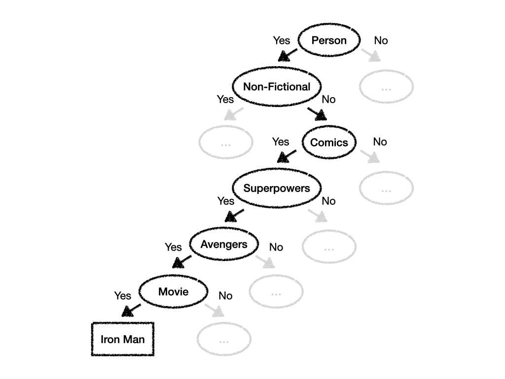
In the image above we can see that the Decision Tree consists of Nodes and Edges which point from parent Nodes to child Nodes. In our case every Node contained a question such as "Is it a person?" while the Edges contained the respective answers: "Yes" or "No". In our case the labels were binary which means that every question can be answered in one of two ways: "Yes" or "No".
While we were playing the game you walked down the tree starting with the root Node at the top, following the Edges and Nodes until you eventually arrived at the Node which had no outgoing Edge: Your prediction.
Generally speaking there are 2 main Decision Tree models both of which differ in the prediction they produce:
The Classification Tree is a tree where the prediction is categorical. The tree we've built above is a classification tree as its output will always yield a result from a category such as "Superheros" or more specifically "Iron Man".
The Regression Tree is a tree in which outputs can be continuous. An example for continuous values are the real numbers.
While this only defines the type of outputs a tree computes there's nothing preventing us from mixing and matching categorical and continuous values in the tree creation phase. Therefore a tree can have categorical as well as continuous Edge labels and output types.
Given what we've learned so far about Decision Trees, it's easy to see that one of the huge advantages is the models understandability. Looking at the trees visual representation it's easy to navigate around, gauge how well it might perform and troubleshoot issues which might arise during real-world usage.
One area of improvement we could identify is the way in which our tree is split. We could've for example skipped the question "Did the person appear in a movie?" since it's highly likely that there's a movie about most of the Avengers. On the other hand nailing that it's Iron Man involved quite some luck. What about Hulk or Thor? It might've been better to insert yet another question to ensure that you're on the right path.
In which way should we construct our tree such that every decision we're making (deciding which Edge to follow) maximizes the information we're getting such that we can make a prediction as accurate as possible? Is it possible to capture this notion mathematically?
Gini Impurity
As it turns out there are a few different mathematical formulas at our disposal to quantify the information we'd gain when following certain paths in our Decision Tree.
One such metric is the so-called Gini Impurity. With Gini Impurity we measure how often we'd incorrectly label a randomly chosen element from our data set if it was randomly labeled according to the class distribution of such data set.
The formula is as follows:
where are the classes and is the probability of picking an element of class at random.
Now if this definition makes your head spin you're not alone. Let's work through an example to understand what we're calculating and how Gini Impurity is used in practice.
Weather Forecasting
Let's pretend that we've collected some meteorology data over the last couple of years and want to use it to determine if we should bring an umbrella with us given the current weather conditions we observe.
Among other things we've collected 14 data points about the wind and temperature:
| Wind | Yes | No | Total |
|---|---|---|---|
| Weak | 4 | 3 | 7 |
| Strong | 6 | 1 | 7 |
| 14 |
| Temperature | Yes | No | Total |
|---|---|---|---|
| High | 3 | 2 | 5 |
| Low | 7 | 2 | 9 |
| 14 |
As one can see we've categorized the wind into "weak" and "strong" and the temperature into "high" and "low". During a day where the wind was "strong" it rained out of times. At the same time it rained out of times when the temperature was "low".
Our goal is to determine which one of these observations provides us more certainty whether it'll rain and therefore if we should take an umbrella with us. We can figure that out by applying the Gini Impurity formula from above.
Let's start with the Gini Impurity calculation for Wind. We're dealing with 2 separate cases here as there can be either "Weak" or "Strong" wind. for every case we have different classes () we can use to label our observation: "Yes" and "No". This means that we need to do Gini Impurity calculations (one for each case). Plugging in the numbers results in the following:
Since we have 2 results (one for each case) we now need to calculate the weighted sum to get the overall result for our Wind observation:
Next up we do the Gini Impurity calculation for Temperature. We're following the exact same steps as we did with our Wind calculation above. We're also dealing with 2 different cases ("High" and "Low") as well as different classes ("Yes" and "No"). Here are the calculation:
Putting it all together we've calculated a Gini Impurity of for our Wind observations and a Gini Impurity of for our Temperature observations. Overall we're trying to work with the purest data possible so we'll decide to go with our data on Wind to determine whether we should bring an umbrella with us.
Building a Decision Tree
In the last section we've learned about a way to quantify purity and impurity of data via a metric called Gini Impurity. In this chapter we'll apply what we've learned so far by putting all the pieces together and build our very own Decision Tree to help us decide if we should play golf given the current weather conditions we observe.
Based on the Gini Impurity metric we'll examine our weather data and split it into different subsets which will reveal as much information as possible as to whether we should go golfing or not. These subsets will be arranged as a tree structure in a way that we can easily trace our decision through it based on our current observations. Our main goal is to come to a conclusion by taking into account as little weather data as possible.
The data set
Let's start by looking at the golf.csv data set we'll be working with:
| Outlook | Temp | Humidity | Windy | Play |
|---|---|---|---|---|
| Rainy | Hot | High | f | no |
| Rainy | Hot | High | t | no |
| Overcast | Hot | High | f | yes |
| Sunny | Mild | High | f | yes |
| Sunny | Cool | Normal | f | yes |
| Sunny | Cool | Normal | t | no |
| Overcast | Cool | Normal | t | yes |
| Rainy | Mild | High | f | no |
| Rainy | Cool | Normal | f | yes |
| Sunny | Mild | Normal | f | yes |
| Rainy | Mild | Normal | t | yes |
| Overcast | Mild | High | t | yes |
| Overcast | Hot | Normal | f | yes |
| Sunny | Mild | High | t | no |
We can see that there are a couple of different features such as Outlook, Temperature, Humidity and Wind we can take into account.
The following command will download the .csv file to our local machine:
wget -O "data/golf.csv" -nc -P data https://raw.githubusercontent.com/husnainfareed/Simple-Naive-Bayes-Weather-Prediction/c75b2fa747956ee9b5f9da7b2fc2865be04c618c/new_dataset.csvNext up we should parse the .csv file and store the result in a structured format. In our case we create a [NamedTuple](https://docs.python.org/3/library/collections.html#collections.namedtuple) called DataPoint in which we'll store one row of information:
golf_data_path: Path = data_dir / 'golf.csv'

class DataPoint(NamedTuple):
    outlook: str
    temp: str
    humidity: str
    windy: bool
    play: bool

data_points: List[DataPoint] = []

with open(golf_data_path) as csv_file:
    reader = csv.reader(csv_file, delimiter=',')
    next(reader, None)
    for row in reader:
        outlook: str = row[0].lower()
        temp: str = row[1].lower()
        humidity: str = row[2].lower()
        windy: bool = True if row[3].lower() == 't' else False
        play: bool = True if row[4].lower() == 'yes' else False
        data_point: DataPoint = DataPoint(outlook, temp, humidity, windy, play)
        data_points.append(data_point)
Notice that we've parsed string such as t or yes into their respective Boolean equivalents.
Our data_points list now contains a dedicated DataPoint container for every .csv file row:
data_points[:5]

# [DataPoint(outlook='rainy', temp='hot', humidity='high', windy=False, play=False),
# DataPoint(outlook='rainy', temp='hot', humidity='high', windy=True, play=False),
# DataPoint(outlook='overcast', temp='hot', humidity='high', windy=False, play=True),
# DataPoint(outlook='sunny', temp='mild', humidity='high', windy=False, play=True),
# DataPoint(outlook='sunny', temp='cool', humidity='normal', windy=False, play=True)]
Some helper functions
Great! We now have the data in a structured format which makes it easier to work with. Let's exploit this structure by implementing some helper functions.
The first function takes an arbitrary data_set and a list of tuples to filter such data_set based on the tuple values:
def filter_by_feature(data_points: List[DataPoint], *args) -> List[DataPoint]:
    result: List[DataPoint] = deepcopy(data_points)
    for arg in args:
        feature: str = arg[0]
        value: Any = arg[1]
        result = [data_point for data_point in result if getattr(data_point, feature) == value]
    return result

assert len(filter_by_feature(data_points, ('outlook', 'sunny'))) == 5
assert len(filter_by_feature(data_points, ('outlook', 'sunny'), ('temp', 'mild'))) == 3
assert len(filter_by_feature(data_points, ('outlook', 'sunny'), ('temp', 'mild'), ('humidity', 'high'))) == 2
*Note: If you're familiar with SQL you can think of it as a SELECT * FROM data_set WHERE tuple_1[0] = tuple_1[1] AND tuple_2[0] = tuple_2[1] ...; statement.*
The second helper function extracts all the values a feature can assume:
def feature_values(data_points: List[DataPoint], feature: str) -> List[Any]:
    return list(set([getattr(dp, feature) for dp in data_points]))

assert feature_values(data_points, 'outlook') == ['sunny', 'overcast', 'rainy']
Those 2 functions will greatly help us later on when we recursively build our tree.
Gini Impurity
As you might've already guessed it we need to implement the formula to calculate the Gini Impurity metric which will help us to determine how pure our data will be after we split it up into different subsets.
As a quick reminder here's the formula:
Which translates to the following code:
def gini(data: List[Any]) -> float:
    counter: Counter = Counter(data)
    classes: List[Any] = list(counter.keys())
    num_items: int = len(data)
    result: float = 0
    item: Any
    for item in classes:
        p_i: float = counter[item] / num_items
        result += p_i * (1 - p_i)
    return result

assert gini(['one', 'one']) == 0
assert gini(['one', 'two']) == 0.5
assert gini(['one', 'two', 'one', 'two']) == 0.5
assert 0.8 < gini(['one', 'two', 'three', 'four', 'five']) < 0.81
Notice the tests at the bottom. If our data set consists of only one class the impurity is . If our data set is splitted our impurity metric is .
We can build a helper function on top of this abstract gini implementation which helps us to caluclate the weighted Gini Impurities for any given feature. This function does the same thing we've done manually above when we've explored our weather data set which consisted of the features Wind and Temperature.
# Calculate the weighted sum of the Gini impurities for the `feature` in question
def gini_for_feature(data_points: List[DataPoint], feature: str, label: str = 'play') -> float:
    total: int = len(data_points)
    # Distinct values the `feature` in question can assume
    dist_values: List[Any] = feature_values(data_points, feature)
    # Calculate all the Gini impurities for every possible value a `feature` can assume
    ginis: Dict[str, float] = defaultdict(float)
    ratios: Dict[str, float] = defaultdict(float)
    for value in dist_values:
        filtered: List[DataPoint] = filter_by_feature(data_points, (feature, value))
        labels: List[Any] = [getattr(dp, label) for dp in filtered]
        ginis[value] = gini(labels)
        # We use the ratio when we compute the weighted sum later on
        ratios[value] = len(labels) / total
    # Calculate the weighted sum of the `feature` in question
    weighted_sum: float = sum([ratios[key] * value for key, value in ginis.items()])
    return weighted_sum

assert 0.34 < gini_for_feature(data_points, 'outlook') < 0.35
assert 0.44 < gini_for_feature(data_points, 'temp') < 0.45
assert 0.36 < gini_for_feature(data_points, 'humidity') < 0.37
assert 0.42 < gini_for_feature(data_points, 'windy') < 0.43
Here is the manual calculation for Humidity:
The Tree Data Structure
We represent our Tree data structure via a Node and Edge class. Every Node has a value and can point to zero or more Edges (out-Edge). It's one of the trees leafs if it doesn't have an out-Edge.
An Edge has a value also and points to exactly Node.
# A `Node` has a `value` and optional out `Edge`s
class Node:
    def __init__(self, value):
        self._value = value
        self._edges = []

    def __repr__(self):
        if len(self._edges):
            return f'{self._value} --> {self._edges}'
        else:
            return f'{self._value}'

    @property
    def value(self):
        return self._value

    def add_edge(self, edge):
        self._edges.append(edge)

    def find_edge(self, value):
        return next(edge for edge in self._edges if edge.value == value)

# An `Edge` has a value and points to a `Node`
class Edge:
    def __init__(self, value):
        self._value = value
        self._node = None

    def __repr__(self):
        return f'{self._value} --> {self._node}'

    @property
    def value(self):
        return self._value

    @property
    def node(self):
        return self._node

    @node.setter
    def node(self, node):
        self._node = node
Building the Tree via CART
We finally have all the pieces in place to recursively build our Decision Tree. There are several different tree building algorithms out there such as ID3, C4.5 or CART. The Gini Impurity metric is a natural fit for the CART algorithm, so we'll implement that.
The following is the whole build_tree code. It might look a bit intimidating at first since it implements the CART algorithm via recursion.
Take some time to thoroughly read through the code and its comments. Below we'll describe in prose how exactly the build_tree function works.
def build_tree(data_points: List[DataPoint], features: List[str], label: str = 'play') -> Node:
    # Ensure that the `features` list doesn't include the `label`
    features.remove(label) if label in features else None

    # Compute the weighted Gini impurity for each `feature` given that we'd split the tree at the `feature` in question
    weighted_sums: Dict[str, float] = defaultdict(float)
    for feature in features:
        weighted_sums[feature] = gini_for_feature(data_points, feature)

    # If all the weighted Gini impurities are 0.0 we create a final `Node` (leaf) with the given `label`
    weighted_sum_vals: List[float] = list(weighted_sums.values())
    if (float(0) in weighted_sum_vals and len(set(weighted_sum_vals)) == 1):
        label = getattr(data_points[0], 'play')
        return Node(label)

    # The `Node` with the most minimal weighted Gini impurity is the one we should use for splitting
    min_feature = min(weighted_sums, key=weighted_sums.get)
    node: Node = Node(min_feature)

    # Remove the `feature` we've processed from the list of `features` which still need to be processed
    reduced_features: List[str] = deepcopy(features)
    reduced_features.remove(min_feature)

    # Next up we build the `Edge`s which are the values our `min_feature` can assume
    for value in feature_values(data_points, min_feature):
        # Create a new `Edge` which contains a potential `value` of our `min_feature`
        edge: Edge = Edge(value)
        # Add the `Edge` to our `Node`
        node.add_edge(edge)
        # Filter down the data points we'll use next since we've just processed the set which includes our `min_feature`
        reduced_data_points: List[DataPoint] = filter_by_feature(data_points, (min_feature, value))
        # This `Edge` points to the new `Node` (subtree) we'll create through recursion
        edge.node = build_tree(reduced_data_points, reduced_features)

    # Return the `Node` (our `min_feature`)
    return node
The first thing our build_tree function does is that it ensures that the list of features we have to examine doesn't include the label we try to predict later on. In our case the label is called play which indicates if we went playing given the weather data. If we find the play label we simply remove it from such list.
Next up we'll compute the weighted gini impurities for all the features in our features list. (Note that this list will constantly shrink as we recursively build the tree. More on that in a minute)
If all our features impurities are 0.0 we're done since we're now dealing with "pure" data. In that case we just create a Node instance with the label as its value and return that Node. This is the case where we end the recursive call.
Otherwise (there's still some impurity in the data) we pick the feature from the weighted_sums dictionary with the smallest score since the smaller the Gini Impurity, the purer our data. We'll create a new Node for this min_feature and add it to our tree. This feature can be removed from our "to-process" list of features. We call this new list (which doesn't include the feature) reduced_features.
Our min_feature``Node isn't a leaf so it has to have some Edges. To build the Edges we iterate through all the values our feature can assume and create Edge instances based on such values. Since the edges have to point somewhere we call build_tree again with our reduced_features list to determine the Node (the next min_feature) the Edges should point to.
And that's pretty much all there is. The function will recurse until it reaches the trees leaf nodes which don't have any outgoing edges and contain the label values.
Let's build our tree with our golf.csv data_points :
features: List[str] = list(DataPoint._fields)

tree: Node = build_tree(data_points, features)
tree

# outlook --> [overcast --> True, sunny --> windy --> [False --> True, True --> False], rainy --> humidity --> [normal --> True, high --> False]]
We can already see the textual representation but it might be a better idea to add a visual representation as well:
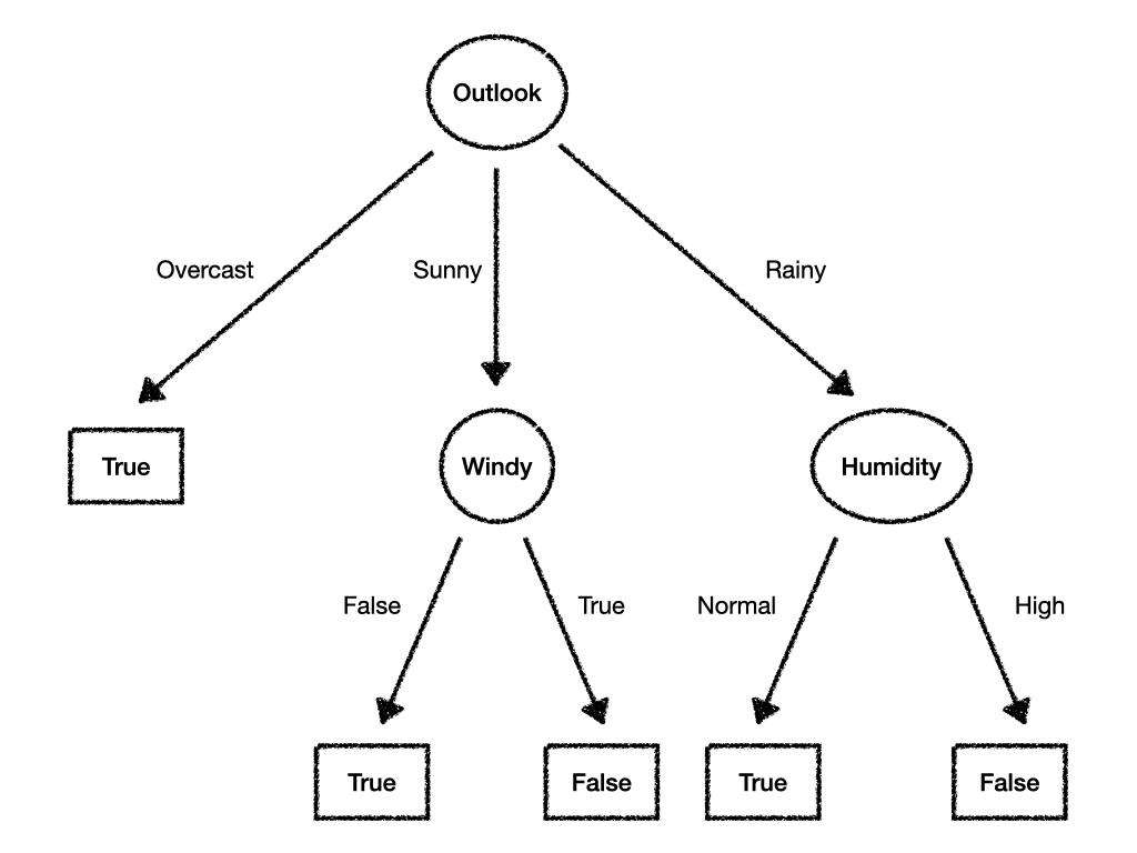
So should we go out when the Outlook is "rainy" and the Humidity is "normal"?
Seems like we've enjoyed playing golf in those situations in the past!
Random Forest
During your journey in the lands of Machine Learning you might come across the terms "Random Forest", "Bagging" and "Boosting".
The problem with Decision Trees is that they tend to overfit easily to the data you train them on. A way to avoid overfitting while also getting better results in general is to build multiple Decision Trees (each with a subset of the training data) and then use them in concert to do predictions.
If you're working with regression trees you'd compute the average of all the trees outputs. If your trees are of categorical nature you'd perform a majority vote to decide which prediction to return.
Combining multiple Decision Trees into one large ensemble is called "Random Forest". Related to Random Forests are the techniques "Bagging" ("Bootstrap aggregation") and "Boosting". But that's for another post.
Conclusion
Everyone of us is confronted with different decision-making processes every single day. Naturally we examine the different scenarios in order to find the best decision we can take given the data we have at hand.
Decision Trees are a class of Machine Learning algorithms which follow the same idea. In order to build an efficient Decision Tree we need to decide the best way to split our data set into different subsets such that every new subset includes as much pure data as possible. Gini Impurity is one metric which makes it possible to mathematically determine the impurity for any data split we attempt.
Using Gini Impurity we implemented the CART algorithm and built our very own Decision Tree to determine if we should play golf based on the current weather conditions.
Given their visual nature, Decision Trees are a class of Machine Learning algorithms which is easy to inspect, debug and understand. On the other hand they also tend to overfit to the data they're trained on. Combining multiple, different Decision Trees into a so-called "Random Forest" mitigates this problems, turning single Decision Trees into a powerful ensemble.
Do you have any questions, feedback or comments? Feel free to reach out via E-Mail or connect with me on Twitter.
Additional Resources
The following is a list with resources I've used while working on this article. Other, interesting resources are linked within the article itself: